Blog

Finite element analyses

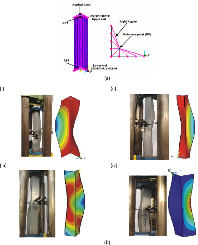
In this study, ANSYS [19.1] was employed to enhance a finite element (FE) model specifically designed for analyzing pin-ended cold-formed steel (CFS) L-columns subjected to axial compression. To accurately represent the structural behavior of these columns, Shell181 elements were used in the FE model. Shell181 elements are 4-noded thin-shell elements that incorporate shear deformation effects, providing six degrees of freedom per node. This element type is known for its comprehensive ability to model complex interactions and deformations in thin-shell structures. The investigation revealed that a mesh configuration with 25 mm² square elements achieved precise results while balancing computational efficiency. This specific mesh size provided an optimal trade-off between accuracy and the computational resources needed, ensuring that the model could deliver reliable predictions without excessive computational demands. The FEA modeling details are shown in Fig. 1(a). A comparison of the failure modes found via finite element analysis (FEA) and experimental tests for structural elements under loading is shown in Fig. 1(b). Figure 1(b) illustrates how well the FEA simulations replicate the failure modes observed in practical tests, with varying configurations and loading scenarios^9,16. This agreement between the experimental and simulation results confirms that FEA is a reliable prediction method for assessing structural failure and stability under compressive loads. Based on the literature, the validation of the FEM is conducted using minimal data^{39,40,41,42,43}.

Section modeling properties and boundary conditions

Elastic-fully plastic material models were used. The values of E and ν were 205 GPa and 0.30, respectively, and four different yield stresses (\(\:{f}_{y}\) = 304.5, 270, 304 and 500 MPa) were used for validation and parametric study. Pin-ended supports were modeled by attaching the ends of the angles to the stiff plates, thus confirming that full secondary warping and local displacement/rotation constraints were provided, which disallowed flexural displacements, major-axis flexural rotations and torsional rotations. Initial geometric irregularities were included in the FE models. Every buckling mode shape was resolved by the resources of an initial ANSYS SFE buckling analysis, which was achieved with exactly the similar mesh employed to accomplish the consequent nonlinear investigation. The first analysis performs a linear buckling analysis to reveal the buckling shape and pattern shapes. The determination of buckling shape should get scaled by using defined factors representing element length percentage or design specification. The nonlinear analysis follows the application of an initial displacement field generated from the scaled imperfection shape. Authorities must check that the initial geometric imperfection magnitude stays within practical values to ensure analysis validity. This technique makes it easy to transform the buckling analysis output into a nonlinear input. No residual stress or corner strength enhancements were built into the FE model; on the basis of the findings of the literature from^9,16,44,45the combined impact of strain hardening, residual stresses and rounded junction properties has a slight influence on the capacity and buckling behavior of CFS L columns.

Confirmation of the FE model

The experimental findings from Cruz et al.^9,16 were used to confirm the FE model established in this study. The axial strengths acquired from the tests of Cruz et al.^9,16 and the FEA accomplished in this study are compared in Table 1. As presented in Table 1, the average ratio of the experimental to FEA results (\(\:{P}_{EXP}/{P}_{ANSYS}\)) is 0.99, with a coefficient of variation (COV) of 0.06. Therefore, the FE models can be used to calculate the strength of the CFS L columns thoroughly.

Parametric study

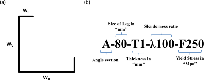
By means of the confirmed FE model, a detailed parametric study was performed to study the influence of different parameters on the axial strength of the CFS L columns (see Fig. 2(a) and Table 2)). The parametrically investigated columns were categorized such that the nominal dimensions of the L leg, section thickness, column slenderness ratio and yield stress were labeled (Fig. 2(b)).

To create a wide range of data points, the following parameters were varied: vertical leg width (W_v) from 80 to 100 mm; horizontal leg width (WH) from 80 to 100 mm; section thickness (t) from 1.2 to 3 mm; yield stress (f_y) from 270 to 500 MPa; and column slenderness ratio (λ) from 20 to 120. The overall width of the lip (WL) and width of the rear lip (WRL) were fixed at 20 mm. In total, 110 FEA models were analyzed, and the FEA results are summarized in Table 4.

DSM design rules

Current design rules^46,47

As per the guidelines outlined in the direct strength method (DSM) for design, the initial design strength without applying factors (\(\:{P}_{D1}\)) for plain sections is determined by evaluating the minimum values of strengths corresponding to flexural buckling (\(\:{P}_{ne}\)), local buckling (\(\:{P}_{nl}\)), and distortional buckling (\(\:{P}_{nd}\)), as demonstrated in Eq. 1.

The equations for computing the strength for flexural buckling (\(\:{P}_{ne}\)) in AISI&AS/NZS^46,47 are shown below:

According to the following formulae, the nominal strength for local buckling (\(\:{P}_{nl}\)) may be determined:

The nominal strength for distortional buckling (\(\:{P}_{nd}\)) can be determined according to the following formula:

where

Equations (2)–(8) involve the gross cross-sectional area represented as \(\:Ag\). \(\:{P}_{crl}\), \(\:{P}_{crd}\), and \(\:{P}_{cre}\) denote the elastic local, distortional, and overall buckling loads, respectively.

Developed design equations

As stated earlier, the FEA model established in this study calculates the axial strength of pin-ended CFS L columns with a high degree of precision. As a result, the results of the parametric study were used to recommend a new design equation in the form of a modified DSM rule for the strength of pin-ended CFS L columns.

The design equation for calculating the axial strength (P_design) of pin-ended CFS angle columns developed in this study is given below:

where

This equation is designed to provide a more accurate prediction of the axial strength by incorporating results derived from FEA, which capture the behavior of these columns under various loading conditions.

Application of the ML models

Extreme gradient boosting (XGB)

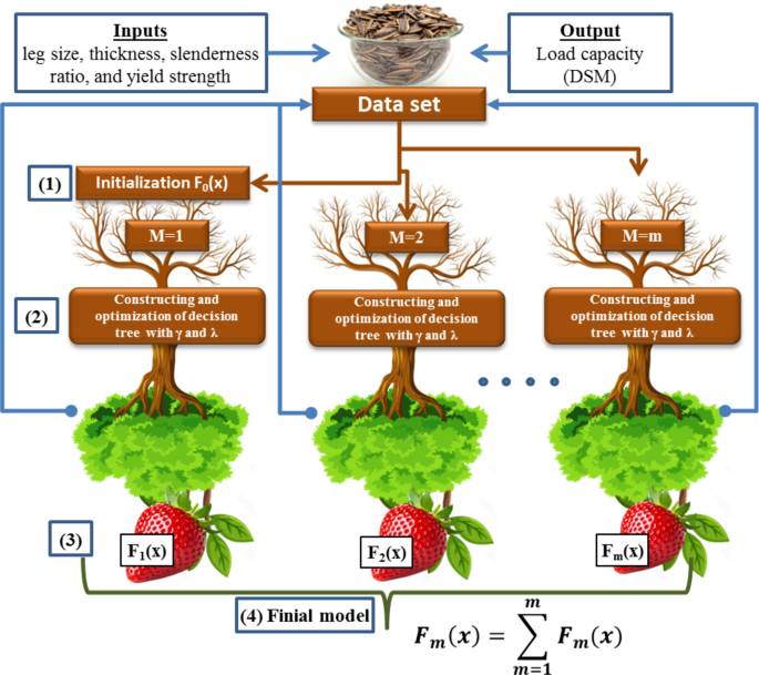
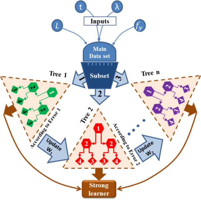
The development of XGB represents a major improvement in artificial intelligence methodologies. The driving force behind the creation of XGB was the need for a scalable tree boosting machine learning model^48,49. The XGB algorithm is based on the decision tree, a popular supervised learning method introduced by Quinlan in 1986⁵⁰ for both classification and regression purposes. It incorporates a regularization term (\(\:\varOmega\:\)) into the differentiable loss function (\(\:L\)) to prevent overfitting and enhance computational performance, speed, and accuracy. It can be expressed below, and the structure of XGB is shown in Fig. 3 using Microsoft PowerPoint 2016.

Here, \(\:{f}_{m}\) represents the weak learner from each individual tree, \(\:\gamma\:\) denotes the minimum reduction in loss, and \(\:\lambda\:\) represents the regularization factor.

The weak learner is

Here, \(\:{g}_{i}\) is the gradient loss function, and \(\:{h}_{i}\) is the Hessian loss function, which is calculated by

Equation (4) can be simplified by eliminating the constant term shown below.

The weight of the \(\:{j}^{th}\) leaf, denoted as \(\:{W}_{j}\) in Eq. (7), can be revised using the optimal weights obtained through

Equation (7) is modified as follows:

Having a similarity score in the first term,

This function is used in the gain function, \(\:{L}_{gain}\), which is used to determine if branching is necessary.

The gain function is expressed as

where \(\:L\) and \(\:R\) are the left and right leaves, respectively, and the weak learners are updated in each leaf:

where \(\:{l}_{r}\) represents the learning rate and \(\:{\varphi\:}_{m}\) denotes the objective function being minimized, which is expressed as

The final combined learner and prediction are acquired by

Adaptive boosting (AB)

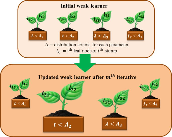
AB is a boosting algorithm that strengthens a learner by linearly combining weak learners and adjusting sample weights through successive regression processes to account for errors in current predictions^48,51. Boosting, as an ensemble method, enhances prediction performance by integrating multiple algorithms rather than relying on a single algorithm. The term “adaptive” in AB indicates its ability to quickly adjust to poorly predicted data and continuously learn predictive models in real time. The AB assigns higher weights to data with larger prediction errors, updating the learning data to better fit the model. Initially, as depicted in Fig. 4 using Microsoft PowerPoint 2016, AB begins with weak learners and iteratively updates them to address their deficiencies, using a varying measure of confidence (α) based on previous performance. The initial weights of the model are expressed below:

The weight varies with respect to the number of data points in the training data (i.e., (x_i, y_i) (i = 1, 2, …, n)). For M equal to one to m, the training process is repeated until the average loss described below is achieved.

Let \(\:{\beta\:}^{\left(m\right)}=\frac{\stackrel{-}{L}}{1-\stackrel{-}{L}}\) represent the confidence level of the weak learner. The updating weight of the data is

On the basis of the learned β(m), each stump is updated to reflect its significance. In this context, m and M denote the index and the total number of weak learners, respectively. The loss for each sample, L_i, is then computed by

where \(\:{F}_{m}\left({x}_{i}\right)\) is the combined weak prediction. The loss function, L, is as follows:

where \(\:D=sup\left|{F}_{m}\left({X}_{i}\right)-{y}_{i}\right|\). The final prediction, \(\:{F}_{M}\left(x\right)\), which results from combining M weak learners, can be represented as

where \(\:{F}_{m}\left(x\right)\) denotes the prediction made by \(\:{m}^{th}\) wesak learner for each input \(\:{x}_{i}\).

Categorical features boosting (CB)

CB is a nonlinear regression technique that employs ensemble learning. It builds on the gradient boosting decision tree (GBDT) framework, which was introduced in 2017⁵². The CB model stands out from other models because of its exceptional ability to automatically manage the encoding of categorical features. GB algorithms often lead to overfitting. This overfitting occurs because the algorithm repeatedly uses the same data in each boosting iteration to reduce model errors, causing estimation deviations^53,54,55,56. CB tackles the overfitting problem commonly associated with gradient boosting by incorporating two key techniques: ordered boosting and gradient-based one-hot encoding (GOHE). At its core, CB constructs an ensemble of decision trees in a sequential manner, where each tree learns from the errors made by its predecessors, and the structure of this booting is shown in Fig. 5.

The algorithm starts with model parameters \(\:M\), training data \(\:{\left({x}_{i},{y}_{i}\right)}_{i=\text{1,2},\dots\:n}\), a learning rate \(\:\alpha\:\), a loss function \(\:L\), and a specified feature order \(\:{\left\{{\sigma\:}_{i}\right\}}_{i=1}^{s}\). It also defines the boosting mode as either plain or ordered. The gradient of the loss function with respect to the model parameters is computed. This involves calculating gradients for each data point, which will guide how the model parameters should be adjusted. A feature is randomly selected for the current tree, which helps to ensure diversity in the model.

The gradient boosting process enhances the prediction of y through a function \(\:{F}^{t+1}\).

where \(\:{h}^{t+1}\)1 represents the base predictor. This predictor is chosen from a collection of functions \(\:H\) to minimize the loss function.

Using either the Taylor series expansion or the negative gradient descent method:

where\(- g^{t} \left( {x,y} \right):\left. {\frac{{\partial L\left( {y,~s} \right)}}{{\partial s}}} \right|_{{s = F^{t} \left( x \right)}} ~\)

However, gradient boosting faces two significant challenges: prediction shift and target leakage. In CB, the fundamental predictors are oblivious decision trees, which are also known as decision tables. The term “oblivious” indicates that the same splitting criterion is applied across an entire level of the tree, leading to a more balanced structure that is less susceptible to overfitting and much quicker during the testing phase. Additionally, CB uses an adaptation of the traditional gradient boosting algorithm known as ordered boosting to prevent prediction shifts and target leakage. This enhances the model’s generalization capabilities, leading to superior performance compared with the leading gradient boosted decision tree implementations such as LightGBM. Furthermore, CB includes the automatic handling and processing of categorical features. To optimize the performance of a CB model, it is crucial to carefully identify and set the relevant hyperparameters before the learning process begins.

After the training algorithm is selected, the fine-tuning phase focuses on identifying the optimal training parameters and the best model structure. The first critical parameter to define is the number of iterations, indicating the maximum number of trees that can be constructed to address the given machine learning problem. Another essential parameter is the maximum depth, which specifies the maximum number of splits in each tree. This value must be carefully chosen: a low maximum depth allows for quick but potentially inaccurate modeling, whereas a high maximum depth might yield a more accurate model but risks overfitting.

To address overfitting, training, validation, and test subsamples were randomly selected, and a 5-fold cross-validation technique was employed. An overfitting detection method was also implemented to halt training if overfitting was detected. Before each new tree is built, the CB algorithm checks how many iterations have passed since the optimal loss function value was achieved. If this number surpasses the set limit for the overfitting detector, training stops. The default threshold for this detector is set at 20 iterations.

Finally, the learning rate, which adjusts the gradient step size during training, must be fine-tuned. The optimal set of hyperparameters was determined on the basis of the loss function value.

Random forest (RF)

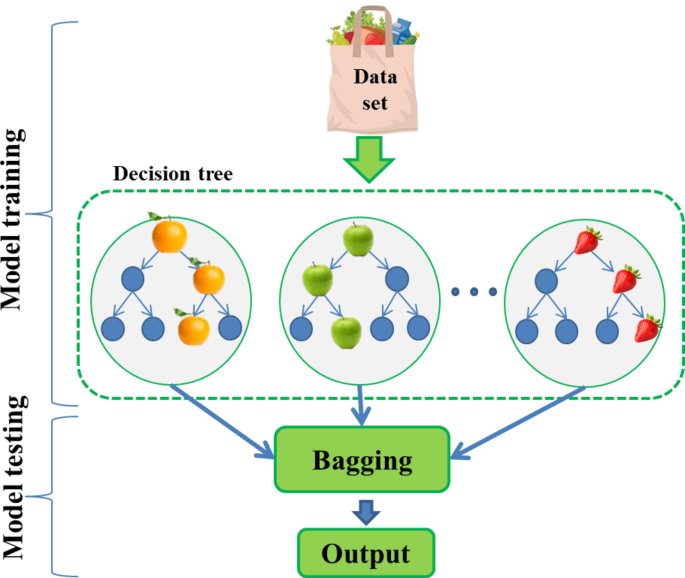
The random forest operates by generating multiple decision trees during the training process. Each tree is built using a randomly selected subset of the dataset and evaluates a random subset of features at each split. This randomness injects diversity into the trees, which helps minimize overfitting and enhances the model’s predictive accuracy. Bagging, introduced by Breiman in 1996⁵⁷, was the initial step in the development of random forest. Later, in 2001, Breiman⁵⁸ expanded on this concept by incorporating a random selection of features, thus defining the random forest algorithm. In prediction, the algorithm combines the outputs of all trees, uses voting for classification tasks and averages for regression tasks. This collective decision-making process, which draws on insights from multiple trees, leads to stable and accurate results. Random forests are popular for classification and regression because they handle complex data well, mitigate overfitting, and deliver reliable predictions in various scenarios^59,60,61.

First, the process involves selecting a subset of data points from the training set. This is achieved by randomly choosing \(\:K\) data points to form the initial subset. Once this subset is established, decision trees are constructed on the basis of these selected data points, creating a series of decision trees tailored to these specific subsets. Next, a predetermined number \(\:N\) is chosen, indicating how many decision trees will be built in total. The procedure of selecting random subsets and constructing decision trees is then repeated to generate multiple trees. In regard to classifying new data points, each decision tree independently provides a prediction. The new data points are ultimately categorized on the basis of the majority vote from all the decision trees, with the category receiving the highest number of votes being assigned to the data points.

The random forest algorithm harnesses the strength of ensemble learning through the creation of multiple decision trees. Each tree in the ensemble acts as a distinct expert, focusing on different facets of the data. By having these trees work independently of one another, the random forest reduces the chance of the overall model being swayed by the peculiarities of any single tree. To guarantee that every decision tree in the ensemble contributes a distinct viewpoint, the random forest algorithm uses random feature selection. When training each tree, a random subset of features is selected. This randomness allows each tree to concentrate on different elements of the data, promoting diversity among the predictors within the ensemble. Bagging, or bootstrap aggregating, is a fundamental method used in training random forest models. It involves generating several bootstrap samples from the original dataset, where instances are sampled with replacement. Each decision tree in the random forest is trained on a different subset of the data, leading to increased diversity among the trees and enhancing the overall robustness of the model. In prediction tasks, each decision tree within a random forest contributes its vote. For regression problems, the final prediction is obtained by averaging the predictions from all the trees. The random forest structure is shown in Fig. 6.

Hyperparameters for the ML models

In this study, an array of machine learning models were meticulously optimized by exploring specific search spaces for their hyperparameters, enabling the selection of the most effective configurations. The RF model emerged as the top performer, achieving optimal results with 110 estimators, no constraints on maximum depth, minimum samples split of 2, and ‘auto’ for max features, indicating a balanced approach to feature selection. The XGB model was fine-tuned to utilize ‘sqrt’ for max features, a max depth of 5, and a learning rate of 0.3, with 100 estimators, a minimum weight of 5, gamma = 0, a subsample ratio of 0.9, a Col sample by tree of 0.8, a regression alpha of 0.1, and a regression lambda of 10, highlighting a sophisticated balance between model complexity and regularization. The AdaBoost model was found to be most effective with 150 estimators and a learning rate of 0.3, reflecting its reliance on iterative boosting for enhanced performance. Finally, the CB model, known for its robustness in handling categorical features, was optimized by selecting a RF as its base estimator. The model was further fine-tuned with 1000 iterations, a learning rate of 0.1, a maximum depth of 4, and an optimized leaf regularization value. This careful tuning of each model underscores the importance of hyperparameter optimization in achieving superior predictive accuracy and model performance.

Data Preparation and preprocessing for the ML models

The models require a sufficient amount of relevant and high-quality data to learn patterns and make accurate predictions. The data are obtained from Table 4, which contains input and output data for estimating the capacity of the CFS columns. In total, 110 data points with inputs are leg size, thickness, slenderness ratio, and yield strength, whereas the data outputs are load capacity (DSM). Normalizing the inputs and output variables in machine learning methods is indeed fundamental for enhancing model accuracy. Normalization (\(\:\text{N}\)) techniques vary depending on the context and the specific requirements of the data^62,63,64. Min–max normalization scales the data to a fixed range, normally among \(\:\left[\text{0,1}\right]\). The expression for min–max normalization is given in Eq. (36). Then, to train and test the model, the normalized data are divided into training data with 77 data points (70%) and testing data with 33 data points (30%).

where N is the normalized value and A is the actual value.

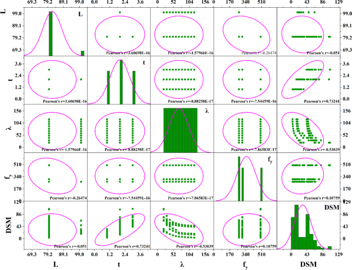
The Pearson correlation coefficient and pair plot of the dataset are shown in Fig. 7, and the results of the statistical analyses are also shown in Table 3.

SHapley additive explanations (SHAP)

SHapley additive exPlanations (SHAP) is a method used to interpret and understand the output by assigning each feature an SHAP value. This value represents the contribution of a feature to a specific output. SHAP values ensure that feature contributions are fairly and consistently allocated to the overall output. By using SHAP, practitioners can gain a clear, interpretable view of feature importance and the relationships between input features and outputs^65,66.

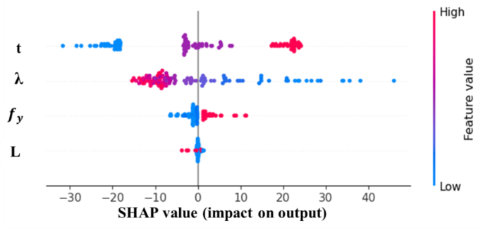
In this section, the data are analyzed to study the impact of the input and output variables. This SHAP plot visually represents (Fig. 8) the impact of different features on the output of the data. The x-axis shows the SHAP values, indicating the extent to which each feature influences the model’s predictions, with positive values increasing the prediction and negative values decreasing it. The y-axis lists the features, labeled \(\:t\), \(\:\lambda\:\), \(\:{f}_{y},\) and \(\:L\), with each feature’s impact depicted as a cloud of points. The color of these points represents the feature’s original value, ranging from blue (low values) to red (high values). This plot reveals that features such as \(\:\lambda\:\) and \(\:t\) have a significant influence on the model’s predictions, as indicated by the widespread of SHAP values. It also shows how higher or lower feature values contribute to increasing or decreasing the model’s output. Overall, the plot provides a clear and comprehensive understanding of feature importance and the nature of its influence on the model’s decisions.

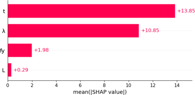
This bar chart represents (Fig. 9) the mean absolute SHAP values for each feature, showing their overall importance in the model. The x-axis indicates the mean of the absolute SHAP values, which quantifies the average impact of each feature on the model’s predictions, regardless of direction (positive or negative). The y-axis lists the features, labeled t, λ, \(\:{f}_{y}\), and L. The chart clearly shows that the features \(\:t\) and \(\:\lambda\:\) have the highest importance, with mean SHAP values of 13.85 and 10.85, respectively. These features have the most significant influence on the model’s predictions. The feature \(\:{f}_{y}\) is less important, with a mean SHAP value of 1.98, whereas \(\:L\) has a minimal impact, with a mean SHAP value of only 0.29. This chart provides straightforward visualization of feature importance, highlighting which variables contribute the most to the model’s decision-making process.

Evaluation of models using performance parameters

The parameters are used to evaluate the performance and quality of the developed algorithm. These metrics are derived from statistical calculations. The coefficient of determination (R²)⁶⁷, root mean square error (RMSE)⁶⁸, performance index (PI), variance account factor (VAF), mean absolute error (MAE), mean absolute percentage error (MAPE), standard deviation ratio (SD), Theil’s inequality coefficient (TIC)⁶⁹ and index of agreement (IA) are all used^70,71,72.

In this context, \(\:{d}_{i}\) represents the observed value for the \(\:{i}^{th}\) data point, \(\:{y}_{i}\) represents the predicted value for the same data point, \(\:{d}_{mean}\) represents the mean value of the actual data, and \(\:N\) represents the total number of data samples. The performance assessment of the models was conducted via Eqs. (37)–(45), and the results were juxtaposed against the ideal values in Tables 6 and 7. Table 6 presents a comparison between the training and testing outcomes of the ensemble models.