
The proposed model for road infrastructure monitoring and analysis is illustrated in Fig. 3. This system integrates various internet-enabled devices, advanced sensors, and YOLOv11-based object detection techniques to collect, process, and analyze data on a wide range of road conditions and anomalies, such as cracks, potholes, faded or missing road markings, snow-covered or uncleared roads, and other structural deficiencies. The model is specifically designed to assess the condition of road infrastructure and evaluate its correlation with overall structure. The architecture is organized into four critical stages: the Data Acquisition, which collects real-time data from the road environment using IoT devices and sensors; the Edge Computing-based Event Categorization Stage, which processes and categorizes events, leveraging YOLOv11 based object detection to accurately identify road anomalies and damages; the Data Mining Stage, which extracts meaningful spatial patterns and insights from the collected data to understand trends and correlations; and the Decision-Making Stage, which utilizes advanced analytics and predictive models to evaluate road infrastructure strength and provide actionable recommendations. Each stage plays a vital role in the system’s functionality, with subsequent stages building upon the outputs and capabilities of the preceding ones to ensure precise and efficient monitoring and analysis of road infrastructure. The overall data flow is depicted in Fig. 4.
Data acquisition
The proposed IoT-based model for road infrastructure monitoring and analysis consists of two key components in the Data Acquisition Stage (DAS). The first component is Data Perception, which employs a network of IoT devices, including environmental sensors, mobile sensors, and smart cameras, to capture real-time data on road conditions, structural integrity, and anomalies such as cracks, potholes, and faded markings. These devices operate using various heterogeneous communication protocols, as outlined in Table 2.
DT formulation for road infrastructure monitoring
The second component of the proposed framework is the Digital Twin (DT) Modulation, designed as a mathematically grounded platform for simulation and predictive assessment of road infrastructure. The DT is modeled as a dynamic virtual mapping of physical road segments, continuously updated from heterogeneous data streams to support real-time monitoring and predictive maintenance planning.
Governing model and data structure
The DT is defined as a functional mapping:
$$\begin{aligned} I(DT,t) = f\left( I_{\text {data}}, I_{\text {SD}}(t), I_{\text {CD}}(t), I_{\text {VD}}(t); \theta \right) \rightarrow Out(t) \end{aligned}$$
With:
-
\(I_{\text {data}}\): Static baseline road information (geometry, layer thickness, elastic modulus, historical interventions),
-
\(I_{\text {SD}}(t)\): Structural sensor measurements at time t (strain \(\epsilon (t)\), deflection \(\delta (t)\), vibration v(t)),
-
\(I_{\text {CD}}(t)\): Contextual variables (traffic load L(t), temperature T(t), rainfall R(t)),
-
\(I_{\text {VD}}(t)\): Visual indicators of surface distress (crack length C(t), pothole density P(t), rut depth U(t)) extracted using YOLOv11 and CNN-BiGRU-based temporal modeling,
-
\(\theta\): Calibrated parameters (learned regression or neural weights),
-
Out(t): Structural indicators (e.g., modulus degradation, crack growth rate) and predicted intervention time.
Deterministic degradation dynamics
The degradation index D(t) (normalized in [0, 1]) is modeled by a differential equation:
$$\begin{aligned} \frac{dD(t)}{dt} = \lambda _1 \, g_1\!\left( I_{\text {SD}}(t)\right) + \lambda _2 \, g_2\!\left( I_{\text {CD}}(t)\right) + \lambda _3 \, g_3\!\left( I_{\text {VD}}(t)\right) – \mu D(t) \end{aligned}$$
where:
-
\(g_1(\cdot ), g_2(\cdot ), g_3(\cdot )\): Feature mapping functions (e.g., linear regression, nonlinear kernels, neural embeddings),
-
\(\lambda _1, \lambda _2, \lambda _3\): Coefficients quantifying contributions of structural, contextual, and visual features,
-
\(\mu\): Recovery factor representing periodic maintenance or self-healing.
The solution D(t) provides a continuous trajectory of road health over time.
Probabilistic transition model
A stochastic Markov chain models discrete health states \(\{H, D, F\}\) (Healthy, Degraded, Failed):
$$\begin{aligned} \textbf{P} = \begin{bmatrix} 1 – \alpha & \alpha & 0 \\ 0 & 1 – \beta & \beta \\ 0 & 0 & 1 \end{bmatrix}, \quad \textbf{s}_{t+1} = \textbf{s}_t \textbf{P}, \end{aligned}$$
where:
-
\(\textbf{s}_t = [p_H(t), p_D(t), p_F(t)]\): Probability distribution over states at time t,
-
\(\alpha = f_\alpha (I_{\text {SD}}(t), I_{\text {CD}}(t))\): Transition rate to degradation, modeled as a logistic function of loads and environment,
-
\(\beta = f_\beta (I_{\text {VD}}(t))\): Transition rate to failure, modeled from observed defect progression.
Integrated prediction framework
The deterministic index D(t) and stochastic state probabilities \(\textbf{s}_t\) are coupled:
$$\begin{aligned} p_D(t) = \mathbb {P}[D(t) \ge \tau _1], \quad p_F(t) = \mathbb {P}[D(t) \ge \tau _2], \end{aligned}$$
where thresholds \(\tau _1, \tau _2\) denote degradation and failure limits, respectively. The output of the DT is expressed as:
$$\begin{aligned} Out(t) = \{D(t), \textbf{s}_t, M(t)\} \end{aligned}$$
with M(t) denoting the predicted maintenance schedule optimized via minimization of expected lifecycle cost.
Validation and calibration
The accuracy of the DT predictions is validated against ground-truth inspection and sensor data. Let \(\hat{y}_i\) be the predicted degradation or distress level at time \(t_i\), and \(y_i\) the observed measurement:
$$\begin{aligned} \mathcal {E} = \frac{1}{N} \sum _{i=1}^{N} \left( y_i – \hat{y}_i \right) ^2, \quad \mathcal {R}^2 = 1 – \frac{\sum _{i=1}^{N} (y_i – \hat{y}_i)^2}{\sum _{i=1}^{N} (y_i – \bar{y})^2}, \end{aligned}$$
where \(\mathcal {E}\) is the Mean Squared Error (MSE) and \(\mathcal {R}^2\) the coefficient of determination.
For state prediction, validation is performed via confusion-matrix-based metrics:
$$\begin{aligned} \text {Accuracy} = \frac{TP+TN}{TP+TN+FP+FN}, \quad F_1 = \frac{2TP}{2TP+FP+FN}. \end{aligned}$$
Parameter calibration is achieved by minimizing the prediction error over \(\theta\):
$$\begin{aligned} \theta ^* = \arg \min _{\theta } \, \mathcal {E}(y,\hat{y}; \theta ). \end{aligned}$$
Thus, the DT is not only predictive but also self-calibrating through continuous data assimilation.
DT simulation
The DT integrates deterministic and probabilistic components:
-
Deterministic simulation The degradation ODE is solved using ordinary differential equation solvers (SciPy.odeint), producing time-dependent degradation trajectories D(t).
-
Probabilistic simulation MCMC sampling (PyMC3) is used to infer \(\alpha , \beta , \lambda _i\), with posterior distributions estimated from observed data. Convergence is ensured using a Gelman-Rubin threshold \(< 1.05\), with 10,000 posterior samples per scenario.
Data integrity and security
Data synchronization between physical and virtual layers is performed using SSL-based transmission. Integrity and access are safeguarded through AES-256 encryption and role-based access control, ensuring compliance with modern cybersecurity standards.
Capabilities of the DT
The resulting DT provides:
-
Real-time integration of multimodal data streams (sensor, contextual, visual),
-
Quantitative degradation trajectories via ODE-based modeling,
-
Probabilistic state predictions through Markov transitions,
-
Predictive maintenance scheduling using learned \(\theta\) parameters,
-
Scalability for large-scale road infrastructure monitoring under varying environmental conditions.
High-level instantiation steps
-
1.
Data onboarding Connect and authenticate data sources (static databases, structural sensor feeds, traffic/environmental APIs, and visual feeds). Verify schemas and apply integrity checks (range checks, timestamps).
-
2.
Preprocessing and feature extraction
-
Clean and align timeseries (resample to common clock, handle missing values with interpolation or model-based imputation).
-
Extract features: from \(I_{\text {SD}}(t)\) compute peak strain vibration statistics; from \(I_{\text {CD}}(t)\) compute moving averages of loads and environmental stressors; from \(I_{\text {VD}}(t)\) run YOLO and CNN-BiGRU pipelines to extract C(t), P(t), U(t) and their temporal embeddings.
-
-
3.
Model initialization
-
Initialize deterministic state D(0) from recent inspection or set to baseline \(D_0\).
-
Initialize Markov state distribution \(\textbf{s}_0 = [1,0,0]\).
-
Initialize parameter priors for \(\theta , \lambda _i, \alpha , \beta , \mu\) to enable Bayesian calibration.
-
-
4.
Calibration (offline/online) Use historical labeled inspections and sensor histories to obtain initial \(\theta ^*\) by minimization of \(\mathcal {E}\). Optionally run an initial MCMC to obtain posterior estimates for uncertainty quantification.
-
5.
Coupled simulation and assimilation loop Start the real-time loop that (i) ingests new data, (ii) updates D(t) via ODE integration over the new interval, (iii) updates \(\textbf{s}_t\) using the transition model with \(\alpha ,\beta\) evaluated using the latest features, (iv) performs parameter assimilation, and (v) emits outputs Out(t) and updated maintenance schedule M(t).
-
6.
Validation and feedback Continuously compute error metrics (\(\mathcal {E}\), \(\mathcal {R}^2\), confusion matrix metrics) on hold-out inspection labels. Trigger model retraining or human review when performance degrades beyond thresholds.
Algorithm 1 presents the overall steps.
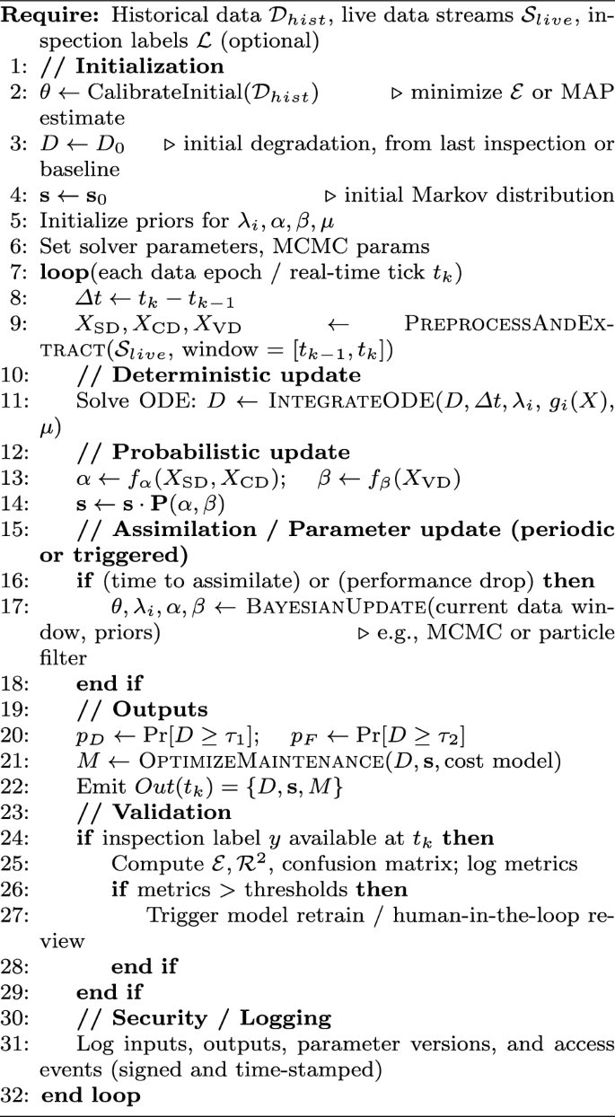
Continuous Digital Twin (DT) Instantiation and Update Loop
Data categorization
Data Categorization plays a crucial role in identifying and notifying relevant stakeholders about abnormal occurrences in real time, particularly in the context of YOLO-based object detection and road infrastructure monitoring. Edge computing acts as an intermediary between the physical layer, where data is collected through IoT devices and cameras, and the cloud layer. Its primary function is to enable immediate detection and response to road infrastructure anomalies. As data, including both physical measurements and visual inputs, is securely transmitted from the physical layer to the cloud, edge computing utilizes a YOLO-based object detection technique to identify irregularities in road conditions. This includes detecting cracks, potholes, faded lane markings, debris, or other structural anomalies in real-time. By processing visual data locally at the edge, edge computing ensures that potential hazards are identified promptly without the need for high-latency cloud processing. Once the edge platform detects any abnormal occurrences, such as significant structural damage or potential safety risks, it immediately triggers alerts and notifications to the appropriate road maintenance teams or authorities. This enables timely intervention and the implementation of corrective measures to maintain road safety and functionality. Edge computing’s real-time response capabilities are critical in road infrastructure monitoring, as they allow for a proactive and efficient approach to managing road conditions. By promptly notifying stakeholders about potential risks or failures, edge computing minimizes downtime, enhances road safety, and prevents further deterioration. This immediate and localized processing ensures a reliable and scalable solution for infrastructure management, leveraging YOLO-based object detection to provide accurate and actionable insights.
Anomaly detection
The proposed study leverages the YOLO model for comprehensive road infrastructure analysis and classification. The YOLO model is specifically chosen for its ability to perform real-time object detection with high accuracy and efficiency, making it particularly suitable for monitoring dynamic and complex environments like road networks. In this study, the YOLO model is applied to analyze visual data captured from smart cameras and other IoT devices deployed across road infrastructure. The model is trained and fine-tuned to detect and classify various road anomalies, including cracks, potholes, faded lane markings, debris, and other structural irregularities. By processing images in a single forward pass, the YOLO model ensures that infrastructure conditions are assessed in real-time, enabling rapid identification of potential hazards. The classification capabilities of the YOLO model go beyond mere detection; it categorizes anomalies based on their severity and type, providing actionable insights for maintenance teams and decision-makers. For instance, the model can differentiate between minor surface cracks and severe structural damage, allowing for prioritized interventions. Additionally, the YOLO model’s ability to process high-resolution images ensures that even small-scale anomalies are accurately detected, contributing to the overall reliability of the analysis.
YOLO-based classification framework with customized technical formulation
Assumptions and indices Let the input image be partitioned into \(S\times S\) grid cells. Each cell \(i\in \{1,\dots ,S^2\}\) predicts B bounding-box candidates indexed by \(b\in \{1,\dots ,B\}\). Let C denote the number of semantic classes. Define the total number of predictions \(N:=S^2 B\). The following notation is used for prediction (i, b):
$$\begin{aligned} b_{i,b} = \big (x_{i,b},\,y_{i,b},\,w_{i,b},\,h_{i,b}\big ), \hat{b}_{i,b} = \big (\hat{x}_{i,b},\,\hat{y}_{i,b},\,\hat{w}_{i,b},\,\hat{h}_{i,b}\big ), \end{aligned}$$
where (x, y) are center coordinates relative to the grid cell, and (w, h) are width and height normalized to the image size. Let \(\hat{C}_{i,b}\in [0,1]\) denote the predicted confidence for (i, b) and \(\hat{P}_{i,b}(c)\in [0,1]\) the predicted conditional class probability \(P(c\mid \text {object})\) (so the per-box class score equals \(\hat{P}_{i,b}(c)\,\hat{C}_{i,b}\)). Assignment indicators:
$$\begin{aligned} \mathbb {1}_{i,b}^{\textrm{obj}} = {\left\{ \begin{array}{ll} 1, & \text { if prediction } (i,b) \text { is assigned to an object },\\ 0, & \text {otherwise}, \end{array}\right. } \end{aligned}$$
Per-box class score For class \(c\in \{1,\dots ,C\}\) the final score for box (i, b) is
$$\begin{aligned} \text {score}_{i,b}(c) \;=\; \hat{P}_{i,b}(c)\,\hat{C}_{i,b}. \end{aligned}$$
Customized loss function (modifications)
The proposed total loss is
$$\begin{aligned} \mathcal {L}_{\textrm{total}} = \lambda _{\textrm{loc}}\mathcal {L}_{\textrm{loc}} + \lambda _{\textrm{conf}}\mathcal {L}_{\textrm{conf}} + \lambda _{\textrm{cls}}\mathcal {L}_{\textrm{cls}}, \end{aligned}$$
with tunable scalar weights \(\lambda _{\textrm{loc}},\lambda _{\textrm{conf}},\lambda _{\textrm{cls}}>0\) and an additional no-object weight \(\lambda _{\textrm{noobj}}>0\) appearing in \(\mathcal {L}_{\textrm{conf}}\) below.
Localization loss (for boxes responsible for objects):
$$\begin{aligned} & \mathcal {L}_{\textrm{loc}} = \sum _{i=1}^{S^2}\sum _{b=1}^{B}\mathbb {1}_{i,b}^{\textrm{obj}} \Big [ (x_{i,b}-\hat{x}_{i,b})^2 + (y_{i,b}-\hat{y}_{i,b})^2 + Y] \\ & Y= \big (\sqrt{w_{i,b}}-\sqrt{\hat{w}_{i,b}}\big )^2 + \big (\sqrt{h_{i,b}}-\sqrt{\hat{h}_{i,b}}\big )^2 \Big ]. \end{aligned}$$
(The \(\sqrt{\cdot }\) terms stabilize gradients for scale.) Confidence loss (object / no-object weighting).
$$\begin{aligned} \mathcal {L}_{\textrm{conf}} = \sum _{i=1}^{S^2}\sum _{b=1}^{B}\Big [ \mathbb {1}_{i,b}^{\textrm{obj}}(\hat{C}_{i,b}-C_{i,b})^2 + \lambda _{\textrm{noobj}}\mathbb {1}_{i,b}^{\textrm{noobj}}(\hat{C}_{i,b}-C_{i,b})^2 \Big ], \end{aligned}$$
where \(C_{i,b}=P(\text {object})\cdot \textrm{IoU}(b_{i,b},b^{\textrm{gt}})\) for the assigned ground-truth box \(b^{\textrm{gt}}\) (or \(C_{i,b}=0\) when no object). Confidence loss (with WIoU replacement). When WIoU is used, replace \(\textrm{IoU}\) by \(\textrm{WIoU}\) in the definition of \(C_{i,b}\). Classification loss (asymmetric weighting, label smoothing). A weighted cross-entropy with label smoothing is recommended to address class imbalance and calibration:
$$\begin{aligned} \mathcal {L}_{\textrm{cls}} = -\sum _{i=1}^{S^2}\sum _{b=1}^{B}\mathbb {1}_{i,b}^{\textrm{obj}} \sum _{c=1}^{C} w_c\,\tilde{y}_{i,b}(c)\,\log \big (\hat{P}_{i,b}(c)\big ), \end{aligned}$$
where \(w_c>0\) is a per-class weight (higher for under-represented defect classes) and \(\tilde{y}_{i,b}(\cdot )\) are smoothed one-hot labels:
$$\begin{aligned} \tilde{y}_{i,b}(c^\star )=1-\epsilon ,\qquad \tilde{y}_{i,b}(c)=\frac{\epsilon }{C-1}\ \text { for } c\ne c^\star , \end{aligned}$$
with \(c^\star\) the ground-truth class and \(\epsilon \in [0,1)\) the label-smoothing parameter. A convenient, tunable penalty is
$$\begin{aligned} \textrm{Penalty}(\delta ) = \exp \big (-\kappa \,\delta ^2\big ),\qquad \kappa >0, \end{aligned}$$
so that small center offsets incur mild penalties while large offsets reduce WIoU more strongly.
Class schema and asymmetric weighting
Four output classes are used:
$$\begin{aligned} \mathcal {C}=\{\textsf {Apt},\ \textsf {Inapt (Crack)},\ \textsf {Inap (Pothole)},\ \textsf {Inap (Other)}\}. \end{aligned}$$
Class imbalance is addressed by setting per-class weights \(w_c\) in \(\mathcal {L}_{\textrm{cls}}\) (e.g., \(w_{\text {Apt}}< w_{\text {Inap (Pothole)}}\)). The vector \(w=(w_1,\dots ,w_C)\) is a hyperparameter to be tuned (via validation or inverse-frequency heuristics).
Training pipeline modifications
The training pipeline incorporates only the following targeted enhancements (standard YOLO training details omitted):
-
Data augmentation Mosaic, CutMix, random cropping/scaling, photometric jitter; ensure augmentations preserve geometric consistency for bounding boxes.
-
Label smoothing Smoothing parameter \(\epsilon\) as above to improve calibration.
-
Class imbalance handling per-class weights \(w_c\) in classification loss or focal-loss replacement:
$$\begin{aligned} \mathcal {L}_{\textrm{focal}} = -\sum _{i,b}\sum _{c} \mathbb {1}_{i,b}^{\textrm{obj}}\,w_c\,(1-\hat{P}_{i,b}(c))^\gamma \,\tilde{y}_{i,b}(c)\log \hat{P}_{i,b}(c), \end{aligned}$$
with focusing parameter \(\gamma \ge 0\) (optional).
-
Confidence target Use \(\textrm{WIoU}\) for \(C_{i,b}\) when greater robustness to center error is required.
-
Optimizer & scheduling Standard choices (SGD with momentum or AdamW), cosine or step LR schedule; hyperparameters selected via validation.
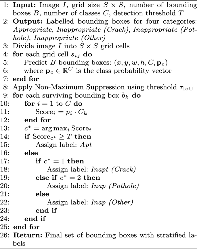
Enhanced YOLO Classification with Custom Label Stratification and Threshold Adaptation
Data mining
Spatial Mining is utilized in road infrastructure analysis to extract and consolidate data across geographical regions based on predefined spatial criteria. The proposed framework is responsible for retrieving spatially distributed data from cloud storage systems. This approach is particularly suited for road infrastructure analysis, as various datasets, such as traffic patterns, road conditions, and environmental factors, are stored with spatial attributes. Spatial mining facilitates data abstraction, enabling the generation of valuable insights by analyzing data from multiple geographical perspectives. This is critical because road infrastructure conditions vary across locations, and capturing spatial diversity is essential. For instance, some events, like monitoring traffic flow or weather conditions, may require high-resolution spatial data, while others, such as detecting road damage or construction activities, may only need localized or regional data. The proposed technique abstracts road infrastructure data using Spatial Patterns, which enables the identification of meaningful patterns and relationships within spatially structured datasets stored in the cloud. By leveraging spatial mining techniques, the proposed model can uncover insights that might not be apparent through non-spatial or static data analysis. The ability to effectively retrieve and analyze spatially structured road infrastructure data from cloud storage is a crucial component of the overall framework, as it provides the foundation for advanced processing and decision-making in subsequent layers, such as predictive maintenance or traffic optimization.
Definition 1
(Spatial Segment) A Spatial Segment in road infrastructure analysis is defined as a set of attributes \((R_l, S_l)\), where \(R_l\) represents a road infrastructure attribute (e.g., road condition, traffic density), and \(S_l\) corresponds to a fixed spatial region \(\delta S\). Here, \((R_l, S_l)\) denotes the attribute \(R_l\) captured by IoT sensors or monitoring devices within the spatial region \(\delta S\). Mathematically, it is represented as:
$$\begin{aligned} {[}R_1, S_1], [R_2, S_2], \dots , [R_l, S_l]. \end{aligned}$$
Definition 2
(Spatial extraction) Spatial Extraction refers to the technique used for abstracting data from structured road infrastructure datasets. It is represented as:
$$\begin{aligned} {[}R_{ab}, R_{ap}], \end{aligned}$$
where \(R_{ab}\) is the abstraction function, and \(R_{ap}\) represents the implication of abstraction for a specific spatial segment.

Spatial extraction procedure.
Key advantages of spatial mining
-
Localized insights Enables the identification of specific regions requiring maintenance or optimization, such as areas with high traffic congestion or frequent road damage.
-
Scalability Facilitates the analysis of large-scale road networks by dividing them into manageable spatial segments.
-
Integration with IoT Leverages IoT-enabled devices to continuously monitor and update spatial data, ensuring real-time analysis and decision-making.
-
Enhanced decision-making Provides the foundation for advanced applications, such as predictive maintenance, route optimization, and resource allocation.
Mathematical representation of spatial mining
The mathematical representation of spatial mining in road infrastructure analysis is as follows:
Spatial segment representation Each spatial segment is defined as:
$$\begin{aligned} S = \{(R_1, S_1), (R_2, S_2), \dots , (R_n, S_n)\}, \end{aligned}$$
Where \(R_i\) represents the road attribute (e.g., road condition, traffic density) and \(S_i\) represents the spatial region.
Spatial abstraction function The abstraction function \(R_{ab}\) is defined as:
$$\begin{aligned} R_{ab}(S) = \int _{S} f(R, S) \, dS, \end{aligned}$$
Where \(f(R, S)\) represents the relationship between the road attribute \(R\) and the spatial region \(S\), and the integral aggregates the data over the spatial region.
Spatial data aggregation Spatial data aggregation is represented as:
$$\begin{aligned} R_{agg} = \sum _{i=1}^n R_i(S_i), \end{aligned}$$
Where \(R_{agg}\) is the aggregated road attribute across all spatial segments. By leveraging spatial mining techniques, the proposed framework enables the effective analysis of road infrastructure data across geographical regions. This approach facilitates localized insights, scalability, and integration with IoT systems, providing the foundation for advanced decision-making in road infrastructure management.
Decision making
Decision-making is employed to predict potential vulnerabilities in road infrastructure. The primary objective is to identify instances where sections of the infrastructure may be at risk due to structural, environmental, or traffic-related factors. By leveraging a hybrid deep learning framework, the proposed system aims to enhance prediction accuracy and reliability. This hybrid approach integrates multiple deep learning architectures to analyze diverse data streams collected from IoT-enabled systems, including environmental sensors, traffic monitoring devices, and structural health monitoring systems. These data streams capture critical information about road conditions, traffic patterns, and environmental factors. Through the combination of deep learning models, the framework is better equipped to identify complex, interdependent patterns that contribute to infrastructure vulnerabilities. For instance, it can detect sudden changes in traffic density, abnormal vibration patterns, or environmental conditions (e.g., extreme weather) that may adversely affect road infrastructure.
Road anomaly assessment
The proposed hybrid deep learning approach for assessing road infrastructure anomalies as represented in Fig. 5, focuses on accurately identifying characteristics that indicate structural or operational risks. The framework utilizes Convolutional Neural Networks (CNNs) to process IoT sensor data collected from the road network over the DT platform. These CNNs are trained to extract features related to potential vulnerabilities and predict their severity levels. The CNN module comprises convolutional and pooling layers, where convolutional layers apply multiple filters to recognize local patterns in raw data signals, and pooling layers summarize these patterns. This architecture enables real-time feature extraction and analysis, improving the system’s ability to identify relevant indicators of road infrastructure risks. However, CNNs alone may struggle to capture long-term temporal dependencies, especially when dealing with extended patterns of traffic flow or structural stress. To address this limitation, the proposed hybrid framework incorporates Gated Recurrent Units (GRUs), a type of Recurrent Neural Network (RNN) designed to model sequential and time-dependent data effectively. GRUs enhance the system’s ability to analyze time-series data, enabling it to learn from complex temporal patterns associated with infrastructure vulnerabilities. By combining CNNs and GRUs, the hybrid framework leverages the strengths of both architectures, resulting in a robust and comprehensive system for predicting potential anomalies.
CNN-BiGRU architecture for infrastructure anomaly detection
The proposed CNN-BiGRU architecture integrates spatial feature extraction and temporal sequence modeling to enhance road infrastructure anomaly detection, as shown in Fig. 6. The CNN module extracts discriminative spatial features from input data, which are then sequentially modeled using a bidirectional GRU (BiGRU) to capture temporal dependencies. This hybrid framework improves detection accuracy, particularly when the training data is limited.
The CNN module processes input images of size \(128 \times 128 \times 3\), applying three convolutional blocks. Each block comprises:
-
A 2D convolutional layer with kernel size \(3 \times 3\), stride 1, and padding 1,
-
ReLU activation,
-
Batch Normalization for stable training,
-
Max-pooling layer with size \(2 \times 2\).
The output of the CNN is a feature matrix:
$$\begin{aligned} F = [f(1), f(2), \dots , f(n)], \end{aligned}$$
where each \(f(i) \in \mathbb {R}^{d}\) represents the feature vector at timestep \(i\), fed into the BiGRU for sequential modeling. The GRU module includes two stacked bidirectional GRU layers, each with 128 hidden units per direction (total 256), using hyperbolic tangent (\(\tanh\)) as the activation and sigmoid (\(\sigma\)) for the gates.
GRU dynamics
$$\begin{aligned} \begin{aligned} r(t)&= \sigma (W_r f(t) + U_r h(t-1) + b_r), \\ z(t)&= \sigma (W_z f(t) + U_z h(t-1) + b_z), \\ \tilde{h}(t)&= \tanh (W_h f(t) + U_h [r(t) \odot h(t-1)] + b_h), \\ h(t)&= z(t) \odot h(t-1) + (1 – z(t)) \odot \tilde{h}(t)). \end{aligned} \end{aligned}$$
The final GRU output \(H = [h(1), h(2), \dots , h(n)]\) is flattened and passed through a Multilayer Perceptron (MLP) with:
-
Dropout layer (\(p = 0.5\)) to prevent overfitting,
-
Dense layer with 64 units and ReLU activation,
-
Output dense layer with 4 units (class labels).
Softmax prediction
$$\begin{aligned} P(t) = \text {Softmax}(W_o h(t) + b_o) \end{aligned}$$
Loss function Weighted categorical cross-entropy is used:
$$\begin{aligned} \mathcal {L}_{\text {cls}} = – \sum _{i=1}^{C} w_i \cdot Y_i(t) \cdot \log (P_i(t)) \end{aligned}$$
where \(w_i\) are inverse-frequency class weights.
Training settings The network is trained using the Adam optimizer (learning rate \(0.001\)), batch size 32, and early stopping based on validation loss.
Data augmentation CutMix, Mosaic, and label smoothing are employed to enhance robustness.

CNN-BiGRU architecture for road infrastructure anomaly detection.


