Extracting signal features and developing the damage index
Several samples with different defect sizes were imaged using Scanning Acoustic Microscopy (SAM). Each sample measured 25 mm \(\times\) 25 mm, and consisted of an aluminum plate containing a predefined defect. When acoustic waves interacted with the sample, they were reflected back and subsequently captured and converted into electrical signals for analysis. The analog signals are converted to discrete-time signals using a digitizer with a sampling frequency of 200 MHz. The transducer’s raster scanning motion was used on the sample surface. In the raster mode, the echo signals are collected at each plate point, and the signal information is recorded. The step size 0.05 mm was used in horizontal and vertical directions, thus acquiring \(100 \times 100\) pixels. Thus, the acquired signals include those resulting from damage (defect) to the plate, which are classified as anomalous, while others represent normal conditions.
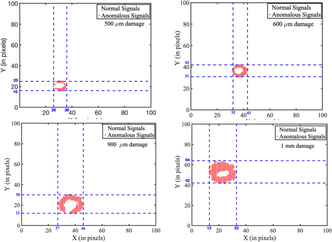
Clustering of anomalous and normal signals using K-means clustering, shown in four subfigures (a–d), representing different defect diameters as indicated in each subfigure. Subfigure (a) corresponds to a defect diameter of (\(500 \upmu m\)), showing a localized anomaly cluster (red circles) near the lower-left region. Subfigure (b) represents a defect diameter of (\(600 \upmu m\)), with a noticeable shift in the distribution of anomalous signals. Subfigure (c) depicts a defect diameter of (\(900 \upmu m\)), showing increased density and spread of anomalous signals across a broader region. Subfigure (d) corresponds to the largest defect diameter of (1mm), where anomalies consolidate into a distinct central cluster. The red circular regions represent cluster boundaries and centroids, illustrating the relationship between defect diameter and the spatial distribution of anomalous signals. Each coordinate in the graph corresponds to a signal at a specific spatial location. Anomalous signals (marked in red) indicate defect regions, while white areas denote normal signals from undamaged positions.
From these signals, features are extracted across the time domain (mean value, RMS value, peak value), the frequency domain (mean frequency, occupied bandwidth, power bandwidth), and the time-frequency domain (spectral skewness, time-frequency ridges). These extracted features are then normalized to acquire our training dataset. The K-means clustering algorithm was then employed to identify anomalous and normal signals based on these features. The experiment was conducted on \(5.05 mm \times 5.05 mm\) aluminum plates with defect diameters of \(500 \upmu m\), \(600 \upmu m\), \(900 \upmu m\), and \(1000 \upmu m\). The results for these 4 samples are shown in Fig. 2. The cluster points are mapped onto their spatial locations, and the maximum pairwise distance among the anomalous cluster points is obtained to find the diameter of the defect. If any outliers were observed, they were ignored in this analysis. The estimated defect diameters are shown in Table 1. The results obtained are very close to the actual diameters.
The estimation error for the largest defect (1 mm) reaches 19%, which is notably higher than for smaller defects. This can be attributed to several technical factors. In SAM, although high-resolution imaging is achievable, the lateral resolution is fundamentally limited by the acoustic wavelength and transducer properties. As the defect size increases, the acoustic signal tends to exhibit more diffuse boundary characteristics, making precise delineation difficult. This results in increased uncertainty during feature extraction and classification. In addition, K-means clustering introduces errors of approximation due to the assumption of spherical clusters with the same variance, which cannot hold for higher-order defects characterized by their irregular and spatially dispersed nature. In this case, signal variability and overlapping decision boundaries reduce the accuracy of estimation. As damage spreads over larger regions, the features may lose sensitivity to small spatial changes. This leads to a decline in classification performance.
In order to address these issues, several improvements are proposed. Applying advanced clustering algorithms such as Gaussian Mixture Models or Density-Based Spatial Clustering of Applications with Noise (DBSCAN) can better capture more complex spatial patterns63,64. Increasing the transducer frequency or incorporating signal deconvolution algorithms can provide higher spatial resolution and tighter borders. Additionally, incorporating spatial correlation features into the feature set offers a promising approach to improving discrimination between larger undamaged regions and long-damaged regions. Together, these advancements can significantly reduce estimation error, particularly for large or irregular defect morphologies.
Surrogate modeling using gamma process
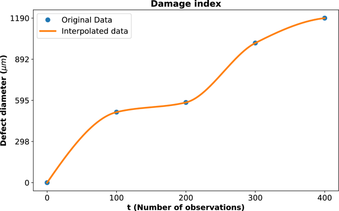
Due to the limited number of data points in the damage index, interpolation was employed to estimate intermediate values. The Piecewise Cubic Hermite Interpolating Polynomial (PCHIP) method was used, as it preserves the shape and monotonicity of the data while providing smooth predictions between existing points. The technique provides a smooth and continuous curve of the damage development, as shown in Fig. 3. For the gamma process modeling, the initial shape parameter value, \(a_0\), was assumed to be 6 and was kept constant throughout the analysis. Similarly, the initial rate parameter (\(b_0\)) was assigned a value of 1. Using these assumptions, the likelihood function was calculated to evaluate the fit of the gamma process to the given data.
Damage index represented by defect diameter (\({\upmu }m\)) as a function of the number of observations. The blue dots indicate the original data points, while the orange line represents the interpolated data using PCHIP. The interpolation provides a continuous representation of the defect diameter progression.
The damage index is represented by defect diameter (\({\upmu }m\)) as a function of the number of observations, as shown in Fig. 3. The deep blue dots indicate the original data points obtained from experimental measurements, which represent discrete instances of observed damage progression. The orange line shows the interpolated data generated using PCHIP, a method chosen for its ability to preserve the monotonicity and shape of the data. The interpolation technique offers a smooth and continuous representation of defect diameter progression. It effectively bridges gaps between sparse data points and enables a more detailed understanding of damage evolution over time.
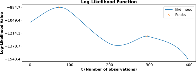
The likelihood function as a function of the number of observations (t). The blue curve represents the computed likelihood values, while the orange markers indicate the identified local maxima at time instants 74 and 293. These maxima correspond to critical change points in the damage progression, highlighting transitions in the structural degradation process and serving as the basis for the two-phase gamma process modeling.
Upon analyzing the complete dataset, the likelihood function revealed two prominent local maxima, as shown in Fig. 4. These peaks occurred at time instants 74 and 293, signifying critical points where the progression of damage exhibited noticeable changes. These time instants, referred to as change points, represent transitions in the behavior of the damage progression, indicating that the process is not uniform over time but instead evolves in distinct phases. To accurately capture these transitions and effectively model the damage progression, a two-phase gamma process modeling approach was employed. The first phase of the gamma process was applied to the time interval spanning from 0 to 293, with the first change point occurring at time instant 74. This phase represents the initial progression of damage, encompassing the behavior both before and after the first significant transition at time 74. The second phase of the gamma process was applied to the time interval from 74 to 400, with the second change point identified at time instant 293. This phase represents the progression of damage following the second major transition at time 293, indicating a distinct dynamic in the degradation process. By dividing the gamma process into two distinct phases, this modeling approach provided a more nuanced and accurate representation of the damage progression over time. The model effectively captured the evolving dynamics of the degradation process, with distinct transitions marked by identified change points. By differentiating between the pre- and post-transition phases, the two-phase modeling approach offers a clearer understanding of how damage accumulates over time. Detecting these behavioral shifts is crucial for enhancing the accuracy and reliability of structural health assessments.
The likelihood function, as illustrated in Fig. 4, represents the computed likelihood values as a function of the number of observations (t). The blue curve shows the variation of the likelihood values across the dataset, while the orange markers highlight two critical local maxima observed at time instants 74 and 293. These maxima are significant as they correspond to change points in the damage progression, indicating distinct transitions in the structural degradation process. The presence of these peaks in the likelihood function suggests that the damage evolution does not follow a uniform pattern but consists of two distinct phases separated by the change points. The first peak at \(t=74\) marks the transition into the initial phase of damage progression, while the second peak at \(t=293\) indicates the onset of a second degradation phase. These change points were instrumental in defining the two-phase gamma process model, which was employed to capture the temporal dynamics of the damage progression accurately. By identifying these critical points, the likelihood function provides a robust method for detecting transitions in structural behavior, enabling more detailed and precise modeling of the degradation process over time.
Real-time updation of the gamma process for prognosis
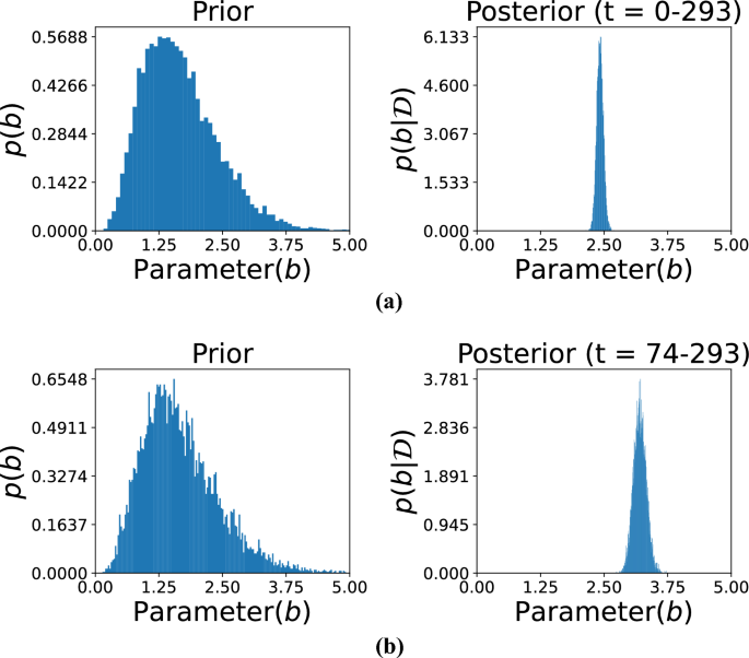
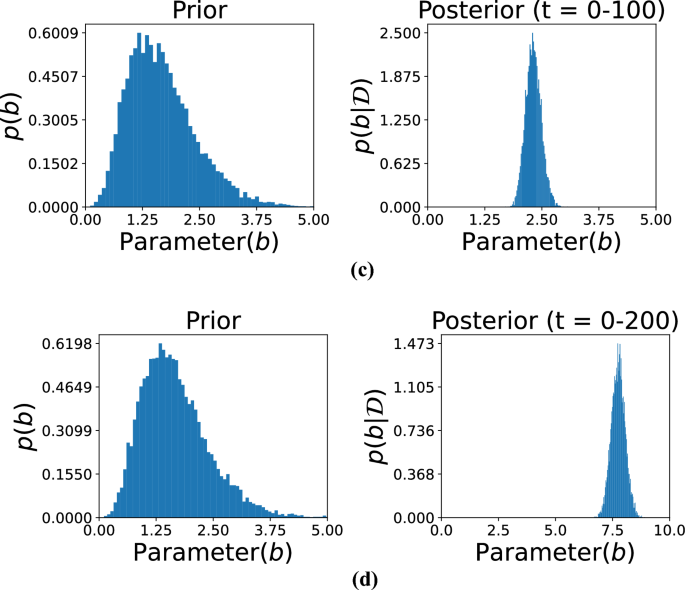
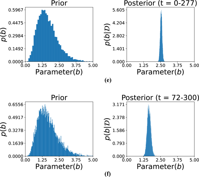
Figures 5, 6, and 7 illustrate the comparison between prior and posterior distributions for the model parameter b, demonstrating the application of Bayesian inference in refining parameter estimates based on observed data across different time intervals. Each figure displays the prior and posterior distributions of \(b\). The prior distribution reflects the initial assumptions, modeled as a gamma distribution with hyperparameters \(\alpha _0 = 5\) and \(\beta _0 = 3\). These parameters define the initial spread and central tendency of the distribution, establishing a prior baseline before incorporating any observed data. The posterior distribution of \(b\), obtained by updating the prior with data from specific time intervals, is also presented. This allows for a refined estimation that reflects both prior knowledge and evidence from actual observations.
The subfigures in these three figures represent different temporal segments that capture distinct phases of the damage evolution process. Specifically, Fig. 5 includes subfigures (a) for time t= 0–293 and (b) for t= 74–293, Fig. 6 includes (c) for t= 0–100 and (d) for t= 0–200, and Fig. 7 includes (e) for t= 0–277 and (f) for t=72–300. These intervals were selected to reflect the evolving nature of structural degradation and allow an assessment of how time-dependent data influences the estimation of the parameter b.
Comparison of the prior and posterior distributions of parameter b across different observation intervals. Subfigure (a) displays the distribution based on observations from 0 to 293, while subfigure (b) focuses on the updated distribution from observations 74 to 293. The comparison illustrates how incorporating new data refines the estimate of parameter b over time.
Shorter observation windows, such as those in subfigures (c) and (d) of Fig. 6, often result in broader posterior distributions. This indicates higher uncertainty due to limited data, which constrains the model’s ability to infer the true parameter values with confidence. In contrast, longer intervals, such as those in Fig. 5, allow for the inclusion of more data points, which sharpens the posterior distribution and narrows the uncertainty. This trend illustrates the principle that increasing the volume of data over time leads to more accurate and confident estimates. Together, these figures highlight the importance of Bayesian inference in damage modeling, where prior knowledge is continually refined through the integration of new data. The shifting and narrowing of the posterior distributions visually and quantitatively emphasize the model’s increasing confidence in the parameter b as more evidence becomes available. Furthermore, the variation in posterior behavior across different time intervals underlines the significance of temporal data selection in predictive modeling. The ability of this approach to adaptively incorporate new information makes it particularly well-suited for structural health monitoring applications, where the degradation process is progressive and dynamic.
Posterior distributions of the model parameter b over large observation time spans. Subfigure (c) presents results based on time steps 0–100, whereas subfigure (d) depicts distributions based on time steps 0–200. These comparisons demonstrate how including more temporal information improves posterior estimation and thus enhances confidence in inferring parameters.
Visualization of the posterior distributions of the parameter evolving b from data covering different periods. Subfigure (e) presents the distribution according to early-period data (0–277), and subfigure (f) presents those from a later period (72–300). The contrast indicates how additional data focuses the estimate of b, monitoring dynamic change in system behavior over time.
The hyperparameters \(\alpha _0\) and \(\beta _0\) for the prior distribution of b were set to 5 and 3, respectively. These hyperparameters determine the shape and scale of the prior distribution, thereby influencing its initial variance and central tendency. As shown in the figure, observational data from specific time ranges were then used to compute the posterior distributions. The subfigures correspond to the following time intervals: (a) t= 0–293, (b) t= 74–293, (c) t= 0–100, (d) t= 0–200, (e) t= 0–277, and (f) t= 72–300. Each time range reflects a different phase of the damage progression, providing insights into how parameter b evolves. The posterior distributions reveal the effect of the observed data in sharpening and shifting the initial assumptions represented by the priors. For instance, shorter time intervals, such as in subfigures (c) and (d), might yield less concentrated posterior distributions due to limited data, leading to broader uncertainty in the parameter estimates. Conversely, longer time intervals, as in subfigures (a) and (b), provide more precise posterior distributions with reduced uncertainty. This progression demonstrates how both the quantity and quality of data contribute to the refinement of parameter estimates. The figure illustrates the dynamic interaction between prior knowledge and observed data within the Bayesian framework. The prior distribution serves as the initial foundation for parameter estimation, while new observations iteratively update this foundation, leading to more accurate and confident results. Moreover, the selection of time intervals significantly influences the resulting posterior distributions, showing how the temporal resolution of data impacts the inference process. This approach is particularly effective for modeling time-dependent phenomena, such as damage progression in structures, where the parameter b captures critical characteristics of the underlying degradation behavior.
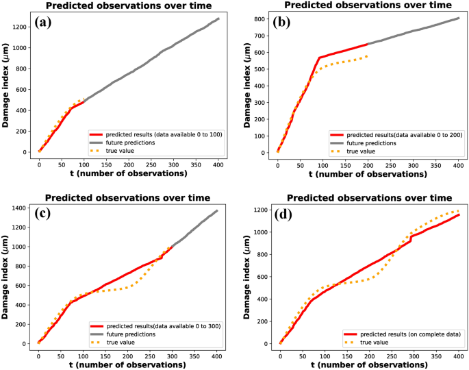
Predicted observations over time using gamma process modeling. The orange dotted curve represents the original data available up to a given time instant. The red curve illustrates the predicted results based on the available data, while the grey curve depicts the predicted future state of the system. Subfigures (a–d) show the predictions for data availability up to \(t= 100\), \(t= 200\), \(t= 300\), and the complete dataset, respectively. The figure demonstrates the accuracy of predictions as the dataset increases in size.
The damage index progression over time was analyzed to evaluate the effect of available data on the accuracy of predictions, as illustrated in Fig. 8. The figure presents four scenarios where the predicted damage index is compared to the true values (\({\upmu }m\)) for varying levels of data availability: (a) data up to \(t=100\), (b) data up to \(t=200\), (c) data up to \(t=300\), and (d) the complete dataset. In each subfigure, the red line represents the predicted results based on the available data, the orange dotted line indicates the future predictions, and the gray line shows the true values. The analysis demonstrates that as more data becomes available, the predictions become increasingly accurate and align more closely with the true damage progression. When the complete dataset was analyzed, two distinct change points were identified at \(t=72\) and \(t=277\). The estimated values of the parameter b from the posterior distributions were found to be 2.42 after the first change point and 3.20 after the second change point (Fig. 8c,d). This indicates that the damage progression exhibited two distinct phases, with a clear transition in the degradation dynamics after each change point. A two-phase gamma process was subsequently applied to model this behavior, effectively capturing the progression over time.
For partial datasets, different observations were made. When data from t = 0–100 was analyzed, a single change point was identified at \(t= 72\), and the parameter b was estimated from the posterior distribution (Fig. 5). Similarly, when data from t = 0–200 was analyzed, a single change point was observed at \(t=93\), with a corresponding parameter value of b obtained from the posterior distribution (Fig. 5f). However, in data from t = 0–300, two change points were identified at \(t= 72\) and \(t=277\), aligning with the results obtained from the complete dataset. These results highlight the impact of data availability on the ability to detect change points and estimate model parameters accurately. With smaller datasets, fewer change points were identified, and the predictions exhibited greater uncertainty, as reflected in the future predictions (orange dotted lines).
As additional data were incorporated, the posterior distributions became increasingly concentrated, resulting in improved estimates of parameter b and more accurate modeling of the damage progression. The value of b was computed as the mean of its posterior distribution. These estimated values were then used to model the system using a Gamma process, capturing the stochastic nature of cumulative damage over time. Figure 8 presents the predicted results and the predicted future state of the system based on this gamma process modeling at various time instants. Figure 8a–c represent the predicted and future damage index up to time instants 100, 200, and 300, respectively. Figure 8d shows the predicted results when complete data is available, closely following the true values. The application of a two-phase gamma process for prognosis provided a robust framework for capturing the non-linear progression of damage over time. This methodology demonstrates the importance of leveraging complete datasets whenever possible to improve the reliability and precision of damage modeling.
Thus, the damage index follows the following distribution on analyzing the complete data from 0–400 :
$$\begin{aligned} \Delta \eta _{jt}&= \eta _{j(t+1)} – \eta _{jt} \sim \Gamma (6 , 1), \quad 0 < t \le 73 \end{aligned}$$
(18)
$$\begin{aligned} \Delta \eta _{jt}&= \eta _{j(t+1)} – \eta _{jt} \sim \Gamma (6, 2.419), \quad 73 < t \le 292 \end{aligned}$$
(19)
$$\begin{aligned} \Delta \eta _{jt}&= \eta _{j(t+1)} – \eta _{jt} \sim \Gamma (6 , 3.203), \quad 292 < t \le 400 \end{aligned}$$
(20)
Figure 8 shows the predicted observations by this gamma process modeling across different time instants.
To quantitatively evaluate the accuracy of the damage prognosis model, a comparison between the predicted and actual damage indices was conducted using Root Mean Squared Error (RMSE) and Mean Absolute Percentage Error (MAPE). Table 2 presents the performance metrics across different partial observation intervals. For forecasts generated using data up to \(t=100\), the RMSE was 80.94 and MAPE was 11.09%, indicating reasonable accuracy during early-stage degradation. When the observation window was extended to \(t = 200\), the RMSE increased to 195.57 and the MAPE to 16.56%, reflecting a temporary drop in performance. This decline may be attributed to evolving damage dynamics that were not yet well captured by the model, possibly due to the use of interpolated data instead of original measurements and the inherent randomness of the gamma process. However, predictive accuracy improved markedly with further data: for \(t=300\), the RMSE decreased to 75.71 and MAPE to 10.60%, while for t=400, the RMSE was 61.59 with a MAPE of 9.99%. These results demonstrate the model’s capacity to generate reliable forecasts with limited initial data, while progressively refining its accuracy as more observations become available. The inclusion of these quantitative metrics strengthens the validation of the proposed unsupervised framework for robust and data-efficient structural health prognosis.
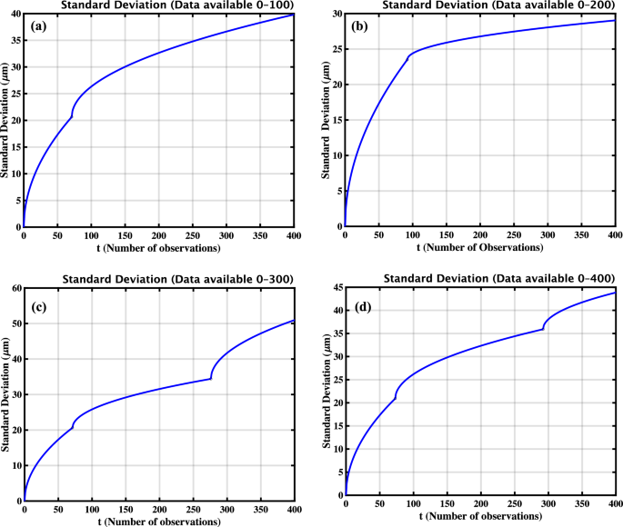
The uncertainty in measurements, or the prediction interval, can be quantified by tracking the standard deviation as more data becomes available. Given that the increments of the damage index follow a Gamma process and are treated as independent random variables, the variance of the damage index at a specific time instant is equal to the cumulative sum of the variances of all previous increments. For a Gamma distribution with shape parameter a and scale parameter b, the variance of each increment is \(a/b^2\). Therefore, the standard deviation of the damage index at time t, accounting for cumulative contributions, is given by60,65,66 :
$$\begin{aligned} \text {Standard Deviation}(\eta _{jt}) = \sqrt{\frac{a}{b^2} \cdot t} \end{aligned}$$
The figures show how the standard deviation changes with time. Let \(\text {Standard Deviation}(\eta _{jt}) = \sigma (t)\)
For data available 0–100 :
$$\begin{aligned} \sigma (t) = {\left\{ \begin{array}{ll} \sqrt{\dfrac{6}{1^2} \cdot t} = \sqrt{6t}, & 0< t \le 71 \\ \sqrt{\dfrac{6}{2.317^2} \cdot (t – 71)} + \sigma (71), & 71 < t \le 400 \end{array}\right. } \end{aligned}$$
For data available 0–200 :
$$\begin{aligned} \sigma (t) = {\left\{ \begin{array}{ll} \sqrt{\dfrac{6}{1^2} \cdot t} = \sqrt{6t}, & 0< t \le 92 \\ \sqrt{\dfrac{6}{7.748^2} \cdot (t – 92)} + \sigma (92), & 92 < t \le 400 \end{array}\right. } \end{aligned}$$
For data available 0–300 :
$$\begin{aligned} \sigma (t) = {\left\{ \begin{array}{ll} \sqrt{\dfrac{6}{1^2} \cdot t} = \sqrt{6t}, & 0< t \le 71 \\ \sqrt{\dfrac{6}{2.546^2} \cdot (t – 71)} + \sigma (71), & 71< t \le 276 \\ \sqrt{\dfrac{6}{1.646^2} \cdot (t – 276)} + \sigma (276), & 276 < t \le 400 \end{array}\right. } \end{aligned}$$
For data available 0–400 :
$$\begin{aligned} \sigma (t) = {\left\{ \begin{array}{ll} \sqrt{\dfrac{6}{1^2} \cdot t} = \sqrt{6t}, & 0< t \le 73 \\ \sqrt{\dfrac{6}{2.419^2} \cdot (t – 73)} + \sigma (73), & 73< t \le 292 \\ \sqrt{\dfrac{6}{3.203^2} \cdot (t – 292)} + \sigma (292), & 292 < t \le 400 \end{array}\right. } \end{aligned}$$
The standard deviation of the damage index is computed over varying amounts of observed data to assess signal stability and damage sensitivity in the PZT sample. Subfigures (a–d) display standard deviation curves calculated using increasing data lengths: (a) 100 observations, (b) 200 observations, (c) 300 observations, and (d) the complete dataset of 400 observations. Each plot illustrates the evolution of standard deviation over time, allowing for a comparison of forecasting uncertainty under different levels of data availability. As additional data are incorporated, the standard deviation increases, reflecting the cumulative uncertainty associated with the progression of the damage index.
To investigate the variability introduced by the stochastic nature of the damage evolution model, the standard deviation of the damage index was analyzed over time. Increments in the damage index are modeled using a Gamma process. As a result, the variance of the damage index increases over time. This is because the variance at any given time is the cumulative sum of the variances of all previous increments. This holds under the assumption that the increments are independent Gamma-distributed variables. Figure 9 illustrates this behaviour by showing standard deviation curves computed using increasing amounts of available data: 100, 200, 300, and 400 observations, corresponding to subfigures (a) through (d), respectively. As expected, the standard deviation of the damage index increases with the number of observations. This reflects the accumulating uncertainty associated with progressive damage over time. The analysis validates the suitability of the gamma process in capturing both the mean trend and the growing variability of the damage index, which is essential for accurate prognosis in structural health monitoring applications.

