Blog

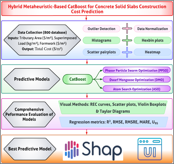
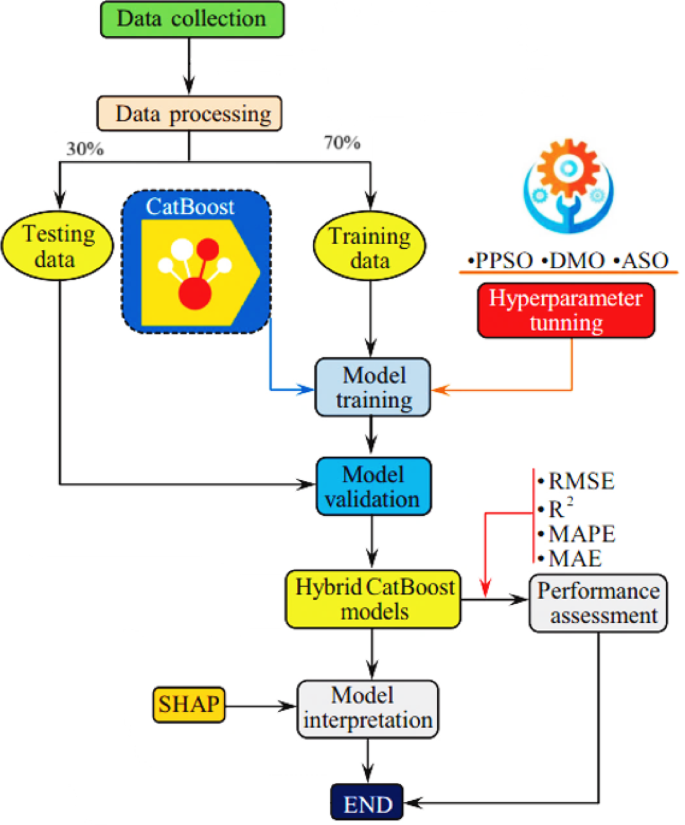
Figure 1 illustrates the methodological framework adopted for predicting the construction costs of concrete slabs using a hybrid machine learning approach. The process begins with data collection and preprocessing, which includes statistical analysis, correlation mapping, and sensitivity evaluation to ensure data quality and relevance. The CatBoost algorithm serves as the core predictive model, with its hyperparameters optimized using three advanced metaheuristic techniques: PPSO, DMO, and ASO. The dataset is divided into training and testing sets to validate model performance. Evaluation is conducted through a combination of visual tools, such as regression error curves and scatter plots and statistical metrics to ensure robust assessment. The methodology concludes with explainability analysis using SHAP to interpret feature contributions and the development of an interactive GUI, facilitating practical application and user engagement. This systematic approach ensures accuracy, interpretability, and real-world usability.

Database collection

The basis of ML methodology is a data set; therefore, the collection of a comprehensive and precise data set is a fundamental step in the development of ML prediction models^33,34. Overall, a database with a sample size exceeding 10–20 times the number of independent parameters used to construct regression models is critical for building reliable and highly generalizable models^{35,36,37,38,39,40,41}. The size, diversity, and quality of the data set are among the key factors affecting the accuracy and performance of ML algorithms. So, the development of an effective ML prediction model includes a meticulous data collection process and a disciplined approach in the analysis phases. This database was used to develop the predictive models in this study. Table 1 lists the collected dataset to ensure reproducibility and practical applicability.

The collected dataset was derived from RSMeans Assemblies and Unit Cost Data Books⁴²covering the period from 1998 to 2018. The dataset includes a total of 800 data instances related to structural floor assemblies, specifically one-way solid concrete slabs used in medium- and high-rise buildings. The dependent variable is the total construction cost of the slab system, expressed in dollars per square meter ($/m²). The input (independent) variables comprise tributary area (m²), superimposed load (kg/m²), unit cost of formwork ($/m²), and unit cost of concrete ($/m³). The year of estimation was not considered an input variable, as the use of multi-year data was solely intended to capture variations in component unit costs across time. RSMeans was selected as the data source due to its comprehensive, annually updated database that reflects current construction material, labor, and equipment costs. It also incorporates new construction methodologies, productivity rates, and localized market conditions to ensure reliability. Independent variables were obtained from the RSMeans Unit Cost Data Book⁴²while the dependent variable was sourced from the RSMeans Assemblies Data Book. This dataset served as the foundation for model development, training, validation, and comparative performance evaluation.

Detection of outliers

Outlier identification using the Interquartile Range (IQR) method is a well-established approach for detecting anomalies in a dataset⁴⁴. This method revolves around analyzing the spread of the data by calculating key percentiles. Specifically, the IQR is the range between the 25th percentile, also called as the first quartile (Q1), and the 75th percentile, called as the third quartile (Q3). The IQR effectively captures the middle 50% of the data, which accounts to the central tendency of the dataset. Equation 1 is used to calculate the IQR.

Once the IQR is calculated, outlier detection thresholds are defined based on extending 1.5 times the IQR beyond Q1 and Q3. These thresholds are represented by the lower and upper boundaries. To determine the lower bound, subtract 1.5 times the IQR from Q1, while the upper bound is calculated by adding 1.5 times the IQR to Q3. The respective equations (Eqs. 2–3) are:

Any data points that fall below the lower bound or above the upper bound are classified as outliers. These outliers are considered to be extreme values that deviate significantly from the rest of the data. Identifying and removing outliers using this method helps in preventing skewing of the analysis or modeling results, as outliers can disproportionately affect calculations like means or regression coefficients.

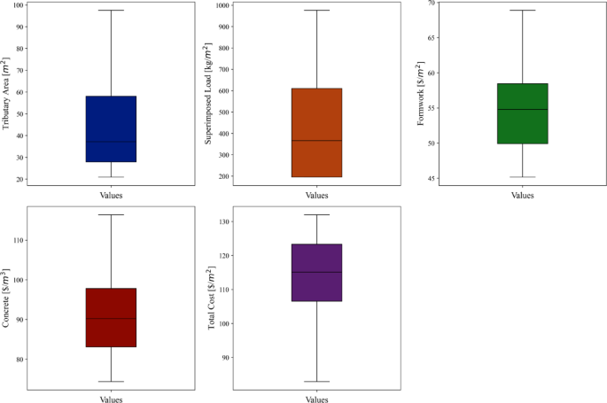
In this study, out of the 800 data points collected for the prediction of the total construction cost of concrete slabs, the outlier detection process using the IQR method identified and removed several extreme data points to create a “cleaned” dataset. After removing these outliers, 704 clean data points remained. This cleaning process ensures that the resulting dataset is free from extreme values, providing a more accurate representation of the true characteristics of the data. To visually confirm that the outliers have been effectively removed, a boxplot illustrating the distribution of the cleaned data is shown in Fig. 2. This figure demonstrates that there are no remaining outliers, ensuring the integrity of the dataset for subsequent analysis, modeling, and insights.

Statistical summary

Table 2 shows the descriptive statistics for various parameters measured in a dataset, highlighting the range, central tendency, dispersion, and distribution characteristics of the variables. The table presents descriptive statistics for a dataset that includes several parameters related to construction costs and load factors. For each of the parameters, key statistical measures such as minimum, maximum, mean, median, standard deviation (Std. Dev.), kurtosis, and skewness are provided. These metrics offer insights into the central tendency, variability, and distribution shape of the data.

The first parameter (Tributary Area, $/m²), shows a minimum value of 20.90 and a maximum value of 97.55, indicating a wide range of data. The mean and median values are 45.91 and 37.16, respectively, suggesting that the data may be slightly skewed towards higher values, as the mean is larger than the median. The standard deviation is 21.89, reflecting considerable variation within the data. The kurtosis is slightly negative at − 0.275, which suggests that the distribution is less peaked than a normal distribution, while the positive skewness of 0.789 indicates a moderate skew towards higher values. For the second parameter (Superimposed Load, kg/m²), the minimum value is 195.28, and the maximum is 976.40, with a mean of 475.23 and a median of 366.15. This difference between the mean and median highlights a potential right-skewed distribution, confirmed by the positive skewness value of 0.732. The standard deviation is 276.68, pointing to a high degree of variability in the dataset. The kurtosis is − 0.744, indicating that the distribution has lighter tails than a normal distribution, which suggests fewer extreme values than expected.

The 3rd parameter (Formwork, $/m²) has a narrower range, with a minimum of 45.15 and a maximum of 68.89. The mean and median are close to each other, at 54.50 and 54.78, respectively, implying that the data is fairly symmetric. This is supported by the relatively low skewness value of 0.442. The standard deviation is 5.74, which indicates moderate variability in the formwork costs. The kurtosis value is − 0.464, showing that the distribution is slightly flatter than normal, but there are no significant outliers or extreme values. For the 4th parameter (Concrete, $/m³), the minimum cost is 74.35, and the maximum is 116.37, with a mean of 90.50 and a median of 90.18. The closeness between the mean and median indicates that the data is approximately symmetric, and the skewness of 0.562 supports this observation. The standard deviation of 9.94 suggests moderate variability in concrete costs. The kurtosis is − 0.162, implying a distribution that is slightly flatter than normal but not significantly different.

Finally, Total Cost ($/m²) exhibits a minimum value of 82.88 and a maximum value of 131.97, with a mean of 114.31 and a median of 115.12. The standard deviation is 11.22, showing moderate variation in the total cost. The kurtosis is − 0.495, which points to a somewhat flatter distribution compared to the normal distribution. The skewness is − 0.458, indicating a slight skew towards lower total costs, although this skew is not pronounced. Overall, the dataset presents moderate variability across the different parameters, with most distributions displaying slight skewness and relatively low kurtosis, suggesting they are generally close to normal but with minor deviations. This analysis highlights the range and distribution characteristics of the various construction-related factors in the dataset.

Histograms

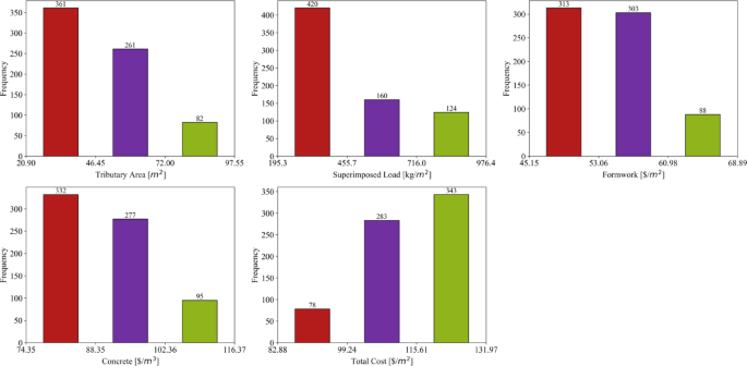
Figure 3 presents a series of histograms that illustrate the frequency distributions of various parameters measured in the dataset. These histograms provide a visual representation of the data, allowing us to observe the distribution patterns and the concentration of values within specific ranges for each parameter. In the first bar chart for Tributary Area ($/m²), the majority of the data points are concentrated in the lower value ranges, with 361 occurrences in the range of approximately 20.90 to 46.45 $/m². This is followed by 261 occurrences between 46.45 and 72.00 $/m², and 82 occurrences in the highest range, between 72.00 and 97.55 $/m². This pattern suggests that most data points for the tributary area fall in the lower value ranges, with fewer instances of higher values, corresponding to the positive skewness noted in the descriptive statistics.

The second bar chart for Superimposed Load (kg/m²) follows a similar trend, where the most frequent values are found in the lower range between 195.3 and 455.7 kg/m², with 420 occurrences. The middle range (455.7–716.0 kg/m²) has 160 occurrences, and the highest range (716.0–976.4 kg/m²) shows 124 occurrences. This distribution is reflective of the positive skew in the dataset, as higher values of superimposed load are less frequent. In the third chart for Formwork ($/m²), the data appears more evenly distributed across the lower and middle value ranges. The range from 45.15 to 53.06 $/m² has 313 occurrences, while the next range (53.06 to 60.98 $/m²) has 303 occurrences. The highest range (60.98–68.89 $/m²) has fewer data points, with 88 occurrences. This indicates a relatively symmetric distribution of values, consistent with the minimal skewness observed in the statistical summary.

The fourth chart for Concrete ($/m³) shows a clear concentration of data points in the lower value range, with 332 occurrences between 74.35 and 88.35 $/m³. The middle range (88.35–102.36 $/m³) has 277 occurrences, while the highest range 102.36–116.37 $/m³) has 95 occurrences. This suggests that most of the concrete costs fall in the lower range, and the distribution has a slight positive skew. Finally, the fifth chart for Total Cost ($/m²) shows a higher concentration of data points in the middle range, with 343 occurrences between 115.61 and 131.97 $/m². The lower range (82.88–99.24 $/m²) has 78 occurrences, while the middle range (99.24 to 115.61 $/m²) shows 283 occurrences. The distribution indicates that total costs are fairly concentrated around the median values, with fewer data points at the extremes. Overall, the figure provides a clear visual representation of how the values for each parameter are distributed, with some parameters showing more skewed distributions (Tributary Area, Superimposed Load) and others displaying more symmetry (Formwork, Total Cost).

Hexbin plots

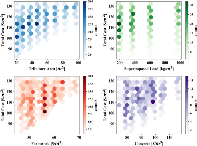
Figure 4 illustrates hexbin plots representing the relationships between total cost per square meter and the four input variables: tributary area, superimposed load, formwork cost, and concrete cost. Each hexbin plot provides a visualization of data density within specific ranges of these variables, with color intensity corresponding to the frequency of data points. In the top-left plot, the relationship between total cost per square meter and tributary area is depicted. The data shows a concentration of costs ranging from $90/m² to $130/m², with tributary areas clustering predominantly between 20 and 100 m². The darker hexagons indicate regions where these cost-area combinations are more frequent, highlighting the distribution of construction projects or designs with typical tributary areas and associated costs. The top-right plot examines the impact of superimposed load on total cost per square meter. Here, costs are distributed across a superimposed load range from 200 to 1000 kg/m², with clear bands of high-frequency data. The consistent vertical alignment of the darker hexagons suggests discrete categories or design constraints influencing superimposed loads in this dataset. The bottom-left plot focuses on the relationship between formwork cost and total cost per square meter. It shows a broad distribution of formwork costs between $50/m² and $70/m², with concentrations in regions where total costs range from $100/m² to $130/m². The denser areas of the plot indicate that variations in formwork costs contribute significantly to the overall construction cost.

Finally, the bottom-right plot captures the relationship between concrete cost and total cost per square meter. This plot reveals a more dispersed pattern, with concrete costs spanning $80/m² to $110/m². The areas of higher density suggest that specific concrete cost levels correlate more frequently with total costs in the $100/m² to $120/m² range, reflecting common material and pricing choices. The plots demonstrate clear patterns and dense clusters for each variable in relation to the total cost per square meter. The structured relationships and well-distributed data points across different ranges of tributary area, superimposed load, formwork cost, and concrete cost suggest that the dataset is comprehensive and exhibits meaningful variability. These characteristics make it suitable for further ML analysis. The density and distribution of the data provide a solid foundation for training predictive models, enabling accurate identification of cost-driving factors and generating reliable predictions for construction cost optimization.

Scatter pair plots

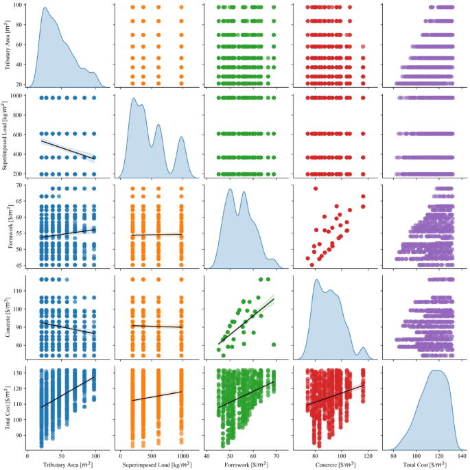
Figure 5 presents a matrix of scatter pair plots with trend lines for the variables in the dataset. Each diagonal of the matrix contains the distribution of each parameter, while the off-diagonal plots represent pairwise scatterplots with regression lines showing the trends between two variables. This visualization allows for a comprehensive view of both the individual distribution of variables and the correlation patterns between them. For the Tributary Area parameter, its distribution shows a heavily right-skewed shape, which indicates that most of the values are concentrated towards the lower end, while only a few observations are found in higher ranges. When paired with other parameters, the scatterplots show some degree of variation. There seems to be a weak positive linear relationship with Total Cost, as indicated by the regression line in the scatterplot between these two variables. However, the other pairwise plots do not show a strong relationship between Tributary Area and other parameters like Superimposed Load, Formwork, or Concrete.

The Superimposed Load parameter shows a multimodal distribution, suggesting the presence of clusters or distinct groups within the data. In the scatterplots with other parameters, the relationship with Total Cost is somewhat weak but still positive, as seen by the slightly upward-sloping regression line. This means that higher superimposed loads are generally associated with higher total costs, though the relationship is not strong. Additionally, the scatterplot with Formwork does not show any noticeable correlation, implying that changes in superimposed load do not significantly affect the formwork cost. The Formwork parameter distribution is more uniform and balanced, reflecting less skew compared to other variables. The pairwise plots with Concrete and Total Cost display moderate positive correlations, particularly with Total Cost, where the regression line shows a clear upward trend. This suggests that increases in formwork costs are associated with corresponding increases in total construction costs. The plot between Formwork and Concrete shows a similar but weaker pattern, indicating that formwork costs may also be slightly associated with concrete costs.

The Concrete parameter displays a relatively symmetric distribution. Its scatterplot with Total Cost reveals one of the strongest positive relationships in the dataset, with a clear upward trend in the regression line. This indicates that higher concrete costs are strongly associated with higher total costs, which makes sense in the context of construction projects where concrete forms a significant part of the total expenditure. The scatterplots between concrete and other parameters, such as Tributary Area or Superimposed Load, show weaker or non-existent correlations. Finally, the Total Cost parameter distribution is shown in the far-right diagonal and follows a slightly right-skewed pattern. The pairwise scatterplots confirm that total cost is moderately to strongly correlated with both formwork and concrete costs, as reflected in the positive slopes of the regression lines. The relationship between Total Cost and the other parameters, such as Tributary Area and Superimposed Load, is positive but weaker in comparison to its relationships with formwork and concrete.

Correlation analysis

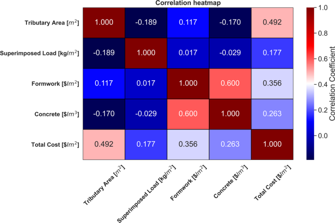
Figure 6 presents the correlation coefficients for the input and output variables. The Tributary Area shows a moderate positive correlation with Total Cost (0.492), indicating that as the tributary area increases, the total cost tends to rise. It has a weak negative correlation with both Superimposed Load (− 0.189) and Concrete (− 0.170), suggesting a slight inverse relationship with these parameters. The correlation with Formwork is weakly positive (0.117). Superimposed Load displays very weak correlations with other parameters. Its relationship with Total Cost is weakly positive (0.177), while its correlations with Formwork (0.017) and Concrete (− 0.029) are near zero, indicating almost no linear relationship with these variables. Formwork shows a moderate positive correlation with Concrete (0.600), implying a notable association between the two variables. The correlation with Total Cost is also moderately positive (0.356), suggesting that higher formwork costs are linked to higher total costs. Concrete exhibits a moderate positive correlation with Formwork (0.600) and a weaker positive relationship with Total Cost (0.263). This suggests that increases in concrete costs are associated with higher total costs, but the relationship is less strong compared to formwork. Total Cost has the strongest correlation with Tributary Area (0.492) and a moderate correlation with Formwork (0.356), followed by a weaker positive correlation with Concrete (0.263). The correlations with Superimposed Load are weak (0.177), reflecting that it has less impact on the overall cost compared to other factors.

Data preprocessing

Multicollinearity and hypothesis analyses

Min–max normalization can help mitigate issues like multicollinearity in regression analysis⁴⁵. This technique is applied using the formula in Eq. (4), as shown below:

In this equation, X_min and X_max represent the minimum and maximum values of the variable, respectively. X_n​ denotes the normalized value of the variable, and X refers to the original variable value being adjusted. This process scales the data to a range between 0 and 1, with the minimum value set to 0, the maximum value to 1, and all other values proportionally distributed within this range. Multicollinearity occurs when predictor variables are highly correlated, making it hard to assess their individual effects. It’s measured using the Variance Inflation Factor (VIF), where values below 2.5 indicate weak multicollinearity and values above 10 suggest problematic multicollinearity^46,47. ANOVA and Z-tests were performed using SPSS to evaluate the impact of input variables on the dependent variable. ANOVA partitions the total variance into regression sum of squares and residual sum of squares, with the total sum of squares representing their sum. The model’s significance is tested using the F-statistic, and a p-value less than 0.05 indicates statistical significance. The Z-test assesses if sample means differ from a hypothesized value, with a p-value below 0.05 suggesting a significant difference.

Sensitivity analysis

Sensitivity Analysis (SA) is a crucial technique for identifying the most influential input variables in predictive or forecasting models⁴⁸. It can be categorized into linear and nonlinear types. This study employs global cosine amplitude sensitivity analysis to determine the key parameters significantly affecting output predictions. The mathematical expression for cosine amplitude sensitivity analysis is given by Eq. (5).

where X_ic is the input parameters, and is X_jk output parameter. An SA value close to one suggests that the independent variable has a strong impact on the output.

Overview of catboost model

CatBoost, short for “Categorical Boosting,” is an open-source gradient boosting library developed by Yandex⁴⁹. It efficiently handles categorical features without extensive preprocessing, utilizing symmetric decision trees for faster training and prediction times. With GPU acceleration, CatBoost reduces training times for large datasets and often outperforms other gradient boosting implementations in accuracy and speed. Its ordered boosting technique minimizes overfitting, enhancing generalization to unseen data. However, CatBoost may require significant memory resources, especially for large datasets with high-cardinality categorical features, and training can be computationally intensive with default hyperparameters. Despite these considerations, CatBoost has been applied across various domains, including recommendation systems, fraud detection, medical data analysis, and sales forecasting⁵⁰.

Description of hybrid catboost models

Figure 7 shows the methodological approach adopted in this study. Firstly, the database was collected, then it was randomly divided into 70% for training and 30% for testing stage. After that, using the training data, the hyperparameters of the CatBoost model were optimized using three different optimization algorithms: Phasor Particle Swarm Optimization (PPSO), Dwarf Mongoose Optimization (DMO), and Atom Search Optimization (ASO), and hybrid models (PPSO-CatBoost, DMO-CatBoost, and ASO-CatBoost) were obtained. The optimization process is computationally demanding. On average, PPSO-CatBoost required approximately 3.5–4 h, DMO-CatBoost about 4–4.5 h, and ASO-CatBoost around 4.5–5 h to complete. These times reflect the need to balance model accuracy and runtime efficiency, especially for large-scale or real-time applications.

The selection of PPSO, DMO, and ASO as optimization techniques is grounded in their proven effectiveness in navigating complex and high-dimensional search spaces, as well as their robustness against becoming trapped in local optima and their flexibility across diverse optimization scenarios^{51,52,53,54,55,56,57}. These hybrid models leverage the strengths of both metaheuristic search and gradient boosting to achieve more refined hyperparameter configurations. Unlike traditional algorithms such as Particle Swarm Optimization (PSO) and Genetic Algorithm (GA), which often require extensive tuning and may suffer from premature convergence or slow exploitation phases, PPSO, DMO, and ASO demonstrate superior convergence behavior, adaptability, and enhanced balance between exploration and exploitation. This makes them particularly suitable for tuning ML models where the search space is non-linear, multi-modal, and sensitive to parameter settings.

PPSO-CatBoost

The original Particle Swarm Optimization (PSO) is a metaheuristic optimization method inspired by animal swarm behavior. It optimizes nonlinear functions by tracking particle movement and minimizing assumptions. In PSO, each particle is defined by its position, velocity, and fitness, and follows both a global optimal and an individual optimal trajectory. The algorithm uses stochastic variables to adjust the particle velocities towards personal best (\(\:pbest\)) and global best (\(\:gbest\)) positions⁵⁸. In PPSO, the phasor angles θ are used instead of constants and arbitrary integers. Additionally, in PPSO, the inertia weight is set to zero. A key advantage of the PPSO algorithm over other methods is its improved efficiency in optimization, even as the problem size increases. In the PPSO algorithm, the position and velocity vectors are denoted by \(\:{X}_{ij}\) and \(\:{V}_{ij}\) (Eqs. 6, 7), respectively, with the velocity vector updated as shown in Eq. (8). Equations (9, 100) were selected after evaluating and testing different functions for PPSO on real test functions by Ghasemi et al.⁵⁹. Subsequently, the updated position of the particle is calculated by adding the velocity vector to its current position, as expressed in Eq. (11):

DMO-CatBoost

DMO algorithm is a newly developed swarm-based metaheuristic method inspired by the behavioral patterns of dwarf mongooses. Unlike other species that create nests for their offspring, dwarf mongooses display a distinctive behavior by relocating their young from one sleeping mound to another, consciously avoiding previously explored areas. This behavior is mimicked in the DMO algorithm, which aims to improve optimization by continuously exploring new solutions and avoiding repetition. The DMO model integrates three distinct behavioral layers that correspond to roles observed in mongoose life: alpha, scouts, and babysitters. In the DMO framework, a cohesive group of mongooses concurrently engages in both exploration of new mounds and foraging activities. As the alpha group initiates its foraging behavior, it simultaneously explores new mounds, intending to move to these locations once the babysitter change criterion is met⁶⁰. The optimization procedure within the DMO begins by initializing the candidate population (X), representing dwarf mongooses⁶⁰. This population is generated by adhering to the problem’s boundary conditions, defined by the lower and upper bounds, as specified in Eq. (12).

where X is the set of current candidate populations, n and d denote the population size and the dimension of the problem, respectively. Then, the fitness value is calculated for each solution and the probability of each individual being alpha is calculated using Eq. (13).

The calculation of the sleeping mound is determined by Eq. (14), and subsequently, the average value of the sleeping mound is computed using Eq. (15).

The movement vector is calculated using Eq. (16). After all, the next position of the scout mongoose is determined using Eq. (17), and these operations are repeated for the maximum number of iterations to obtain the best solution.

where phi and rand are a uniformly distributed random number [− 1, 1] and a random number between [0, 1], respectively.

ASO-CatBoost

Atom Search Optimization (ASO) is a novel physics-based metaheuristic algorithm designed to solve global optimization problems. The ASO algorithm operates by simulating basic molecular dynamics, specifically focusing on the interactions between atoms and their neighboring atoms. These interactions are modeled by considering both attractive and repulsive forces from neighboring atoms as well as constraint forces from the best atom (i.e., the best solution). The algorithm creates a model of atomic motion based on these forces⁶¹. The primary objective of the ASO algorithm is to optimize the value of the fitness function by determining the atom’s velocity and position, while accounting for its mass and the forces acting on it. The mass of each atom is first calculated using Eq. (18). After that, the algorithm identifies K neighboring atoms with better fitness values according to Eq. (19).

where \(\:{m}_{i}\left(t\right)\), N, \(\:Fi{t}_{best}\), and \(\:Fi{t}_{worst}\) are the mass of the i-th atom, number of atoms in the population, and fitness values of the best and worst atoms at the i-th iteration, respectively.

where T is the maximum number of iterations. The interaction forces (attract or repel) and constraint force acting on the atom are calculated using Eqs. (20, 21), respectively.

where \(\:{K}_{best}\) is a subset of an atom population consisting of atoms with the best fitness value, \(\:{rand}_{j}\), \(\:\beta\:\), \(\:{x}_{best}\), and \(\:{x}_{i}\) denote a subset of an atom population consisting of atoms with the best fitness value, a random number in [0, 1], the multiplier weight, the position of the best atom, and the position of the i-th atom, respectively. The acceleration of the atom is determined by substituting the calculated forces and mass into Eq. (22), and the position of the atom is determined using Eqs. (23, 24), respectively. This process is repeated until the best fitness value is determined⁶¹.

where \(\:{v}_{i}\) and \(\:{x}_{i}\) are the velocity and position of the i-th atom.

Parameters of the proposed algorithms

In this study, the hyperparameters of the CatBoost model were fine-tuned using three recent metaheuristic optimization algorithms: PPSO, DMO, and ASO, to enhance model performance. As a result, three hybrid frameworks combining CatBoost with each optimization technique were established. The integration of these optimizers into the CatBoost tuning workflow was achieved using the open-source Mealpy Python module⁶². CatBoost, a Python-based gradient boosting library, was employed for model construction. The internal settings of each optimizer listed in Table 2 based on recommendations by their respective developers⁵⁷. The target hyperparameters optimized include the model’s depth (ranging from 1 to 10), learning rate (0.01 to 0.10), and number of iterations (100 to 1000), due to their known impact on prediction accuracy. The optimization process focused on minimizing the Root Mean Square Error (RMSE) by efficiently exploring these parameter ranges.

Evaluation criteria

The evaluation of predictive models is fundamental to establishing their scientific credibility and practical applicability⁶³. While training datasets assess a model’s capacity to fit the provided data, testing datasets are crucial for evaluating its ability to generalize to unseen data, mitigating overfitting and enhancing its applicability in real-world scenarios. This study adopts a dual evaluation approach, incorporating both visual and quantitative methods^64,65. Visual tools, such as scatter plots, facilitate the analysis of the relationship between predicted and actual values, enabling the identification of patterns and anomalies that may not be evident through numerical measures. Quantitative evaluation, on the other hand, employs numerical metrics to objectively assess accuracy and reliability^66,67, forming the basis for model comparison and selection⁶⁸. Furthermore, uncertainty analysis is conducted to assess the robustness and reliability of the models⁶⁹. Quantitative metrics play a pivotal role in providing objective and reproducible evaluations of model performance. Such measures are extensively used in research for rigorous model assessment and comparison⁷⁰. In this study, six key metrics were selected to ensure a comprehensive evaluation: R², RMSE, RMSRE, MAE, MAPE, and U₉₅. These metrics, detailed in Table 4, offer valuable insights into the predictive accuracy, error magnitude, and reliability of the constructed models, facilitating the identification of the most effective predictive framework for the given task.

Feature importance analysis

Interpreting machine learning models is crucial for assessing their effectiveness⁶⁵. SHAP is a popular method for feature sensitivity analysis, helping to understand how each input feature influences predictions. Derived from game theory, SHAP assigns an “importance value” to each feature by calculating its marginal contribution across different subsets of inputs. SHAP provides local interpretability, explaining individual predictions, which enhances transparency. Its consistency and additivity make it a reliable tool for analyzing feature importance in complex models.