Blog

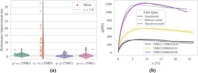
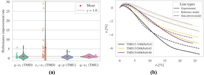
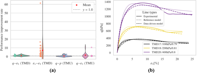
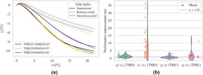
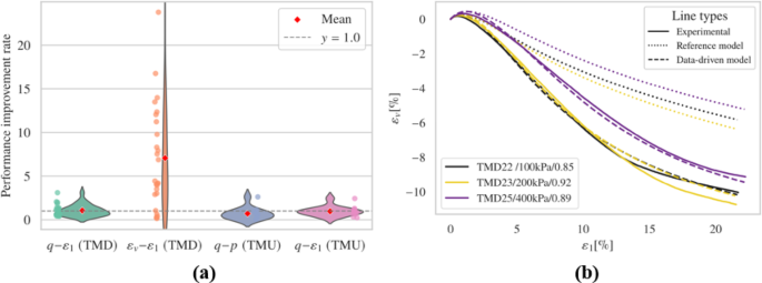
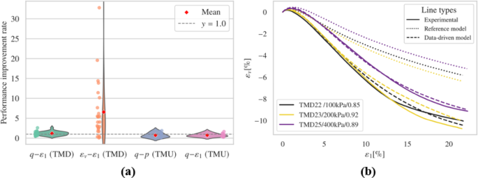
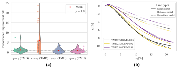
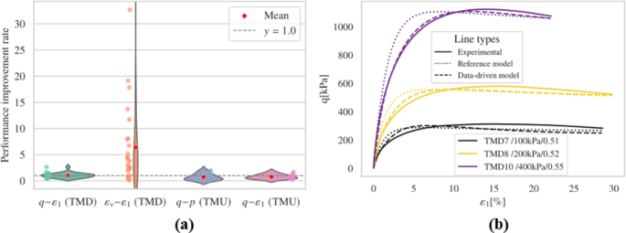
For each fine-tuned model, finite element simulation software was utilized to simulate 25 different drained triaxial experiments, 6 undrained triaxial extension tests, and 6 undrained triaxial compression tests, all based on experimental conditions documented in the database⁵⁶. In all the graphical representations that follow, solid lines denote experimental records, dotted lines represent simulations using the reference model’s UMAT, and dashed lines correspond to simulations with the fine-tuned model’s UMAT. Identical colors indicate the same simulation; labels such as TMD1/50 kPa/0.2 refer to the experiment’s name (e.g., TMD1 indicates triaxial monotonic drained test numbering 1, TMU1 indicates undrained triaxial monotonic test numbering 1), initial confining pressure (50 kPa), and initial relative density (0.2), using the naming conventions from the dataset⁵⁶.

As mentioned in Sect. 2, convergence ability and compliance with physical phenomena are crucial when implementing a data-driven constitutive model in FEM simulations. An evaluation procedure tailored for granular constitutive models is then introduced and described below. Table 2 illustrates this procedure in detail.

The extrapolation ability can be checked through the performance of data-driven UMAT in FEM simulations. To quantify this, the convergence ratio can be defined as the proportion of successful FEM simulations that reach the target loading relative to the total number of simulations conducted. For example, the convergence ratio is 0.5 if only half of the simulations successfully converge to the designed target loading.

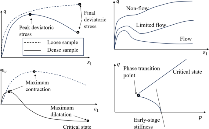
As for the adherence to crucial physical phenomena, this can be evaluated by whether the constitutive model can reproduce crucial phenomenon observed in experiments, as shown in Fig. 7. These phenomena include but are not limited to (1) the ability to reflect critical state in drained and undrained tests under large deformation; (2) limited flow and flow in undrained tests; (3) phase transition in undrained test.

As for the fitting ability, we need to quantify the difference between simulation records and experimental records. The sampling frequency in numerical simulations often differs from that in experimental measurements, leading to inconsistencies in data resolution. This mismatch may result in numerical simulations having more or fewer data points than their corresponding experimental datasets. Consequently, traditional regression loss metrics, such as mean absolute error (MAE) or the \(\:{R}^{2}\) coefficient, cannot be directly calculated. To address this, the dynamic time warping (DTW) algorithm is employed to robustly compare temporal sequences that may be misaligned. DTW is widely used to quantify mismatches between numerical and experimental curves. Prior to comparison, all curves are normalized based on experimental data, as illustrated in Fig. 2.

Then the effectiveness of fine-tuning, which aims to enhance performance beyond that of the pre-trained model, can be evaluated using the average improvement ratio defined as:

where \(\:{N}_{c}\) is the number of curves for comparison (the number of triaxial simulations); \(\:{W}_{ref,i}\) indicates the normalized DTW distance between the experimental results and those from the reference model for the \(\:i-\)th curve, and \(\:{W}_{nn,i}\) is the normalized DTW distance between the experimental results and those from the data-driven model for the \(\:i-\)th curve. A larger value of \(\:\stackrel{-}{{W}_{rel}}\) indicates that the DTW distance of the data-driven model is significantly lower than that of the reference model, implying a better fit to the experimental data. Moreover, the notation \(\:\stackrel{-}{{W}_{rel}}\left(q,p\right)\) indicates that the discrepancy is evaluated based on the \(\:q-p\:\)plots.

Influence of fine-tuning configurations

In transfer learning, to preserve knowledge acquired by the pre-trained model and to adapt to the scarcity of target data⁵⁷, it is common practice to use its parameters as initial values while keeping some parameters fixed throughout the training process⁵⁰, meaning some parameters are “frozen.” This section explores how the way of freezing parameters influence outcomes. To minimize confounding variables such as data volume, this analysis specifically highlights the effects of parameter freezing by expanding the test set to include 15 TMD tests (selecting three randomly per relative density level) and 8 TMU tests (four each from extension and compression experiments selected randomly). Additionally, this section compares the impact of different loss terms and batch sizes used during the fine-tuning process. Fine-tuning was conducted over 3000 epochs, with other parameter configurations maintained as per Table 1.

Freeze the first layer

The results obtained from freezing the input layer’s weights and biases, followed by fine-tuning with experimental data, are shown in this section. For brevity, only representative cases and overall performance are presented in Fig. 8. Complete records are available in the supplementary material.

The fine-tuned model generally predicts the timing and magnitude of peak deviatoric stress more accurately than the reference model in drained triaxial simulations. Regarding dilatancy evaluation, the fine-tuned model exhibits notable improvement in capturing the general \(\:{\epsilon\:}_{v}-{\epsilon\:}_{1}\) trend and the evolution of void ratio when compared to the reference model. However, irregular trends were noted in the \(\:{\epsilon\:}_{v}-{\epsilon\:}_{1}\) plots for several simulations, including TMD 1, TMD 5, TMD 11, and TMD 16. Figs. S3 and S4 display the effective stress paths and stress-strain relationships for all undrained simulations. Compared to the reference model, the fine-tuned model achieves commendable results but produces unrealistic negative pressures in the TMU 7 and TMU 11 simulations, leading to a convergence problem.

Freeze the first two layers

Freezing the weight matrices and bias vectors of both the input layer and the first hidden layer, the fine-tuned model has only 91 adjustable parameters. The effects of considering only the loss \(\:{E}_{r}\) associated with \(\:dT\) and introducing additional error terms \(\:{E}_{a}\) were explored, along with the impacts of batch size and learning rate adjustments. The model underwent 3000 epochs of training, maintaining other configurations as per Table 1.

Consider only \(\:{E}_{r}\)

Figure 9 and Figs. S5-S6 show outcomes of drained test simulations. When considering only \(\:{E}_{r}\), the model’s performance in predicting deviatoric stress under dense conditions and at higher confining pressures was not as accurate as the reference model. Although the fine-tuned model showed better volumetric behavior, it produced physically unrealistic rapid contraction behaviors at the end of loading for TMD 25.

The fine-tuned model outperforms the reference model in undrained simulations, particularly evident in the \(\:q-p\:\)relationships as depicted in Figure S6. Specifically, the fine-tuned model successfully captured limited flow, which is not effectively reproduced by the reference model. However, anomalies occurred in the TMU 11 simulation, where unrealistic tensile states (\(\:p\:\)< 0) led to non-convergence issues. Interestingly, in several simulations such as TMU 3, TMU 5, and TMU 6, the results closely aligned with the reference model, indicating that retaining more parameters from the pre-trained model can yield performances similar to the reference in certain aspects.

Consider only \(\:{E}_{a}\)

If only the loss component \(\:{E}_{a}\) is included in the fine-tuning process, the outcomes are displayed in Fig. 10 and Figs. S9-S12. Overall, its visual performance exceed that of using only \(\:{E}_{r}\). However, it does not encounter convergence issues, and the quantitative analysis pre sented in Sect. 4.1.4 reveals certain advantages.

Incorporate further loss items

When additional loss term \(\:{E}_{a}\) is included in the fine-tuning process, the outcomes are displayed in Fig. 11 and Figs. S13-S16.

The introduction of an additional loss term, \(\:{E}_{a}\), in the fine-tuning process resulted in improved predictions of deviatoric stress, although the volumetric behavior in simulations of loose samples occasionally exhibited suboptimal performance. The undrained test results, as illustrated in Figs. S15 and S16, showed slight degradation; the \(\:q-p\) curves effectively reflected initial stiffness but struggled to identify the phase transition points accurately, although they did reflect the critical state line. The deviatoric stress responses over the strain development were similar to those models considering only \(\:{E}_{r}\), with several simulations aligning closely with the reference model. However, the inclusion of additional constraints contributed to greater stability, preventing convergence issues and physical inaccuracies.

Effect of batch size

The choice of batch size influences MLP performance yet selecting the most suitable batch size and learning rate for optimal generalization remains unclear⁵⁸. Typically, the effects of batch size and learning rate are discussed with respect to specific datasets⁵⁹ or particular tasks⁶⁰, which aids in building well-performing models. The interaction between batch size and learning rate is crucial⁶¹. Generally, a smaller batch size can help achieve global optima in clean data sets, which is why a smaller batch size of 32 was initially used for the calibration of the pre-trained model (refer to Table 1). In this section, a departure from the small batch size and learning rate listed in Table 1 is taken, opting instead for a larger batch size (2048) combined with a lower learning rate (1e-4), with the results depicted in Fig. 12 and Fig. S17-S20.

Following the introduction of the additional loss term \(\:{E}_{a}\) and the use of a larger batch size with a smaller learning rate, the performance in drained test simulations was further improved. The behavior in undrained tests remained largely unchanged, still capturing initial stiffness well but failing to accurately capture phase transition points, although the critical state line was still evident.

Further checking on the architecture

Further checking was carried out by altering the network structure, including freezing more neurons and freezing all parameters of the pre-trained model while incorporating additional neural layers. New layers were added both before and after the original output layer, effectively reprocessing the \(\:{p}_{i}\) parameters (\(\:i\)=1,2,3) of the reference model. Results indicated that freezing more parameters improved convergence but reduced the model’s fitting performance. Adding new layers worsened outcomes due to decreased flexibility, although this led to more stable convergence and smoother curves in finite element simulations. For brevity, detailed results are presented in the supplementary information.

Combining the findings from this section, it is clear that moderately freezing parameters (as demonstrated by freezing the first two layers), adopting more comprehensive constraints, and adjusting batch size and learning rate according to data quality can significantly enhance the overall performance of the model.

Performance comparisons

All models discussed in this section are compared based on their convergence ability under different boundary conditions, adherence to physical phenomena, and curve-fitting performance. The results are presented in Table 2.

Overall, the fine-tuned model outperforms the reference model in drained simulations and generally provides improved predictions of the \(\:q-{\epsilon\:}^{1}\) relationship under undrained conditions. However, it shows reduced accuracy when predicting the \(\:q-p\) relationship under undrained conditions. Results indicate that using both \(\:{E}_{r}\) and \(\:{E}_{a}\) loss terms is more effective than using a single loss term, resulting in the most significant performance improvements compared to the reference model. Additionally, increasing the batch size brings the model’s performance closer to that of the reference model. Retaining more trainable parameters improves curve-fitting but adversely affects convergence. Therefore, in subsequent studies, the parameters of the first two layers are kept fixed, and both \(\:{E}_{r}\) and \(\:{E}_{a}\) loss terms are employed during training.

Limit available data

To emphasize the assumption of limited laboratory data, the experimental setup was limited to five drained triaxial tests (TMD) and two undrained triaxial tests (TMU). Specific initial conditions for the drained tests were \(\:\left({p}_{0},{I}_{d0}\right)\)= (200 kPa, 0.21); (300 kPa, 0.55); (50 kPa, 0.57); (100 kPa, 0.79); (25: 400 kPa, 0.95). For the undrained tests, initial conditions were \(\:\left({p}_{0},{I}_{d0}\right)\)= (200 kPa, 0.64); (200 kPa, 0.53). This design involved multiple initial relative densities and confining pressure levels but only one sample per level, replicating the constraints found in real-world testing conditions. The undrained compression and extension tests (axial stretching) also occurred in only one set, covering a very limited range of variables, representing the practical scenarios where only a few tests might be conducted.

Two scenarios were considered: the first excluded any synthetic data from undrained simulations; the second used simulated undrained experiments using the reference model to supplement the drained experiment data records with stress-strain data obtained from simulations. Based on findings in the previous sections, this part of the model froze the first two layers and considered both \(\:{E}_{r}\) and \(\:{E}_{a}\) during the calibration process. Given the limited number of available drained experiment records, a larger batch size than in previous sections could not be employed; thus, a batch size of 960 was used, while keeping other parameters unchanged from earlier settings.

Without synthetic data

The results from the drained simulations (Fig. 13 and S21-S22) indicate that a significant reduction in available data somewhat negatively impacted model performance. While the development of deviatoric stress did not show substantial differences, this suggests that capturing shear stress in drained conditions may be comparatively less sensitive to data availability. However, the volumetric behavior was notably affected, with poor simulation outcomes under lower initial confining pressures (50 kPa). The undrained simulations (Figs. S23-S24) were also affected, with the most notable issues occurring in the triaxial extension tests involving loose samples, where excessive shear stress development was observed.

With synthetic data from undrained simulation

To address the excessive accumulation of shear stress observed in undrained triaxial extension simulations when only two undrained experimental tests were available, this section augmented the dataset with synthetic data. In addition to the two original undrained test records, ten extra undrained tests were simulated using the reference model. However, only data from the final portion of these simulations, namely the part where axial extension or compression strain exceeded 70% of its final value, was used to fine-tune the model. This approach aims to minimize the contamination of experimental data by low-fidelity synthetic data, while preserving informative samples that lie at or near the critical state. The results of this approach are presented in Fig. 14 and Figs. S25-S28.

Incorporating this additional undrained test data did not meaningfully affect the outcomes of the drained simulations, neither enhancing nor reducing the model’s performance in terms of deviatoric stress development or volumetric behavior.

For the undrained simulations, while the results of the undrained compression tests remained largely unchanged, the excessive growth of shear stress in the undrained extension tests was effectively alleviated. This adjustment highlights the potential benefits of selectively expanding the training dataset to address specific modeling challenges without substantially affecting the overall performance.

Use only drained tests

This section investigates in more detail the implications of drastically limiting the available dataset for calibrating the PeNNs. In this scenario, the assumption is that merely five drained experimental records are available. Given the further reduction in available data, a batch size of 320 is selected to accommodate the smaller dataset.

Without synthetic data

When only five drained experimental records are available for fine-tuning the models, the results of the triaxial test simulations are shown in Fig. 15 and Figs. S29-S32. The simulation outcomes for drained tests are comparable to the results in the previous section, indicating that excluding undrained experimental data does not significantly impact the simulation of drained tests, especially regarding volumetric behavior. However, the prediction of shear stress was negatively impacted, showing a reduction in performance under conditions of higher initial confining pressure.

In terms of undrained simulations, despite the absence of undrained experimental records in the fine-tuning dataset, the simulations of undrained compression tests still performed well. Nevertheless, the simulations of undrained extension tests showed unphysical shear strength loss when axial extension was significant, highlighting the necessity of including drained extension test data for accurate modeling.

With synthetic data of undrained test

Similar to the approach detailed in Sect. 4.2.2, this section incorporates synthetic data generated by undrained simulations to fine-tune the PeNNs.

The outcomes of the drained test simulations are depicted in Fig. 16 and Figs. S33-S34. The introduction of synthetic undrained data has significantly enhanced the performance of the model in predicting deviatoric stress in drained tests. However, there were no significant changes observed in volumetric behavior.

The simulation results for undrained tests, as shown in Figs S35-S36, indicate a clear improvement compared to models trained solely on drained experiment data. The inclusion of even partial undrained test data strongly improves the simulation results for undrained extension tests, closely matching the experimental trends. This confirms that synthetic data can effectively supplement limited real data. This is particularly beneficial in scenarios where experimental data are are limited or expensive, enabling robust model performance even with very limited real-world data.

Influence of data in fine-tuning process

To investigate the impact of the available experimental data volume and the incorporation of synthetic data on the fine-tuned models, we compared models fine-tuned with different datasets under identical conditions. Specifically, we analyzed the models presented in Sect. 4.1.2.3, Sect. 4.2.1 and 4.2.2, and Sect. 4.3.1 and 4.3.4 and summarized the results in Table 3.

As shown in Table 3, a reduction in available experimental records visibly diminishes the performance of the fine-tuned models. Introducing synthetic data appropriately can mitigate this decline. When the available experimental data includes only a minimal number of undrained test records, the model’s simulation performance deteriorates, exhibiting issues such as non-convergence, inability to capture limited flow behavior, and reduced fitting accuracy. If the available data contains no undrained test records, the model’s convergence substantially worsens, fails to accurately reflect the critical state, and even produces unrealistic collapse behavior in undrained extension simulations.

However, incorporating synthetic data during the fine-tuning process can enhance model performance. For instance, Model 4.3.1, which does not include any synthetic or experimental data related to undrained behavior, is unable to simulate phase transition point in undrained extension simulation, as clearly demonstrated in the resulting figures. This indicates poor extrapolation capabilities. However, quantitative analysis reveals that Model 4.3.1 performs better in undrained conditions compared to the model discussed in Sect. 4.3.2, which includes synthetic undrained data. Even when using an alternative similarity metric, the Fréchet distance, Model 4.3.1 outperforms the model 4.3.2 (0.87:0.77 for \(\:q-p\) plots and 0.72:0.72 for \(\:q-{\epsilon\:}_{1}\) plots). However, this quantitative superiority does not correlate with the actual performance observed.

These comparisons highlight that relying solely on quantitative metrics for fitting ability is insufficient. It is essential to first evaluate the convergence behavior of FEM simulations and the adherence to physical phenomena. In scenarios with limited experimental data, the introduction of synthetic data during fine-tuning can enhance both the convergence performance and the physical accuracy of the models.