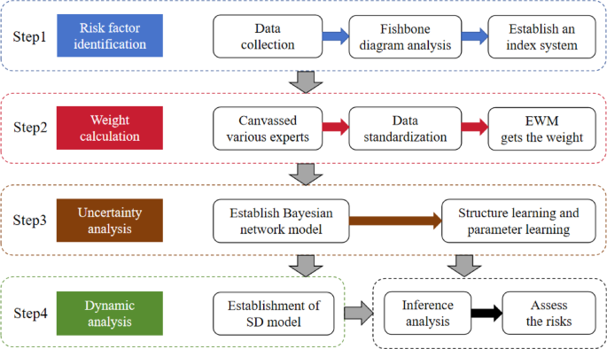
This paper obtained data through questionnaire survey. After referring to the official website of the State Department of Emergency Management, the China Safety Production Network and the Code for Safe Construction of Geological Drilling (DB37/T11-2022) [Local standard of Shandong Province], the index system was determined by using fish-thorn map. After the drilling construction safety risk assessment index system was established, the expert scoring method and entropy weight method are used to assign and weight the risk factors in the index system, and evaluate the safety risk of each index. Then, the Bayesian network model is established according to the index system, the risk probability of each index is calculated, and the safety risk of drilling construction is further evaluated. Then the system dynamics model is established using the weights given by the entropy weight method. For a dynamic assessment of drilling construction safety risks, Fig. 1 illustrates the various stages of the research process, including data collection and analysis, development of models, and risk assessment in case studies.
Data source
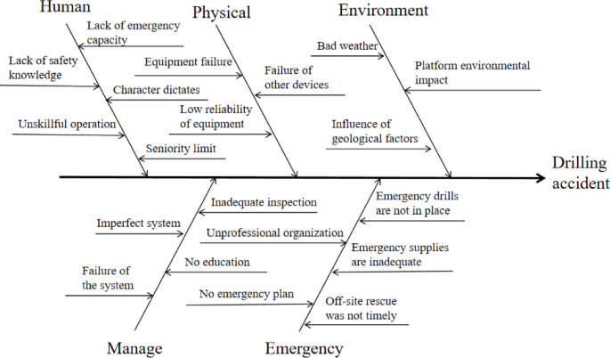
Drilling construction safety assessment is to ensure the safety of drilling process, which usually covers drilling equipment and facilities, drilling equipment installation, drilling site electricity, safety protection, site management and other aspects. The Code for Safe Construction of Geological Drilling (DB37/T1811-2022) [Local Standard of Shandong Province]30 provides relevant codes and standards. According to this standard, this paper determines five sub-risks in the index system: human, physical, environment, manage and emergency.
With reference to the cases published on the official website of the Ministry of Emergency Management and the China Production Safety Network31, the risk indicator system based on five sub-risks, human, physical, environmental, management and emergency response, was drawn through the analysis of actual cases.
Fishbone diagram analysis
In the risk analysis of drilling construction, through structured classification, the potential risk factors are systematically identified, the causal chain of accidents is visually displayed, and the team is helped to focus on the core causes and formulate targeted preventive measures, thus improving the systematic and comprehensive risk prevention and control. As shown in Fig. 2 below.
Index weight
According to the questionnaire survey method, five questionnaires were sent to 25 experts and scholars respectively, and the obtained data were returned to the experts after processing. In this way, continuous and complete data were obtained after three rounds of repetition, so as to carry out statistics on the data of the indicator system. A total of 20 evaluation indexes from C1 to C20 of the five sub-risks of human, physical, environmental, management and emergency response were obtained. Among them, a score above 80 was considered as high risk, a score between 60 and 80 was considered as medium risk, and a score below 60 was considered as low risk. However, for the problem of missing data, when dealing with missing data in Bayesian network parameter learning, we can use list deletion (for a small amount of MCAR data), data filling (such as mean or model prediction), expectation maximization (EM algorithm, Iterative optimization of parameters), Bayesian methods (such as MCMC joint estimation of parameters and missing values), or multiple filling (taking uncertainty into account), where non-random missing (MNAR) requires explicit modeling of missing mechanisms (such as the introduction of indicator variables); Method selection requires a balance of missing mechanisms (MCAR/MAR/MNAR), computational resources, and uncertainty requirements, often combining EM preliminary estimates with Bayesian refinement, or balancing efficiency and accuracy with a tool library such as pgmpy. The expert weight can be obtained by the following formula:
$$W_{{\exp {\text{ert}}}} { = }\frac{{\overline{s}_{i} }}{{\sum\nolimits_{k = 1}^{n} {\overline{s}_{k} } }}$$
The entropy weight method is used to determine the weight of drilling construction safety risk evaluation index32, and the weight of five aspects of drilling construction risk including human, physical, environment, manage and emergency is determined by information entropy. Calculate the information entropy of five indexes of drilling construction risk: human, material, environment, management and emergency, the information entropy Ej for the j attribute is:
$$E_{j} = – \frac{1}{\ln n}\sum\limits_{i = 1}^{n} {p_{ij} } \ln p_{ij}$$
In the formula: n indicates the number of indicators; \(p_{ij} = \frac{{z_{ij} }}{{\sum\nolimits_{i = 1}^{n} {z_{ij} } }}\), zij is the normalized attribute value, i indicates the sequence number of the sample object, i = 1, 2, …, n; j = 1, 2, …, m.
The attribute importance of the j attribute Dj can be defined as:
The weight calculated by the entropy weight method and the weight scored by the expert are fused using the addition average:
$$W_{final} = 0.5W_{expert} + 0.5W_{entropy}$$
Uncertainty analysis
The construction of a reasonable and complete Bayesian network mainly includes the following three aspects: the determination of Bayesian network structure, the determination of basic information of network nodes, and the determination of Bayesian network parameters33.
In this paper, the Bayesian network node represents the risk factors affecting the safety of drilling construction, and the state of each node is described as the risk size. Each node has three states, namely HIGH (H), MEDIUM (M) and LOW (L), indicating the HIGH (H), MEDIUM (M) and LOW (L) of the impact of risk factors on the safety of drilling construction. Under normal circumstances, the prior probability of each node can be obtained through questionnaire survey.
Qualitative analysis and quantitative evaluation are the two main parts of Bayesian network model. Qualitative analysis and quantitative evaluation can be carried out in three ways: modeling by using expert knowledge, modeling by using existing data, and modeling by combining expert knowledge and machine learning34. Because there are many risk factors affecting the safety of drilling construction, the modeling method combining expert knowledge and machine learning is used to construct the model.
Bayesian network structure learning
Bayesian network structure learning methods are mainly divided into two categories: Bayesian network structure learning based on conditional independence test and search-based scoring method. K2 algorithm and mountain climbing method are two classical algorithms commonly used in search-based scoring methods. Taking human factors as an example, the optimal algorithm is selected for subsequent application through comparison experiments. The results of the two algorithms after parameter learning are compared as shown in Fig. 3 below.
It can be seen from the results that there are differences between the two algorithms, because K2 algorithm can directly constrain the network structure through domain knowledge, so as to avoid generating dependency relationships that do not conform to professional logic. However, mountain climbing method only relies on greedy search of scoring function, which may fall into local optimality and cannot be directly integrated into a prior causal order. In drilling construction risk assessment, K2 algorithm realizes polynomial time complexity in computing efficiency through node sequence constraint and greedy search strategy, which is suitable for processing tens of variables in engineering scenarios. In terms of accuracy, its structure guidance based on domain knowledge and anti-overfitting characteristics of BDe score can generate a risk causal network with high confidence. This paper uses the Bayesian network analysis software GeNIe2.1 to construct the highway safety risk assessment model by K2 algorithm35. The calculation process of K2 algorithm mainly includes the following two aspects:
-
(1)
Structure scoring function.
It is assumed that the nodes of Bayesian network structure have the same prior probability, the recorded data are independent and equally distributed, no data is lost in the data set, and each variable in the structure is a discrete variable36,37. Based on these four assumptions, the scoring function is:
$$p\left( {G_{B} ,D} \right) = p\left( {G_{B} } \right)p\left( {\left. D \right|G_{B} } \right) = p\left( {G_{B} } \right) \cdot \prod\limits_{i = 1}^{n} {\prod\limits_{j = 1}^{{q_{i} }} {\frac{{(r_{i} – 1)!}}{{\left( {N_{ij} + r_{i} – 1} \right)!}}} } \cdot \prod\limits_{k = 1}^{{r_{i} }} {N_{ijk} } !$$
Among them, The range ofXi \(\left\{ {x_{i}^{1} , \ldots ,x_{i}^{{r_{i} }} } \right\},\) \(N_{ij} = \sum\limits_{k = 1}^{{r_{i} }} {N_{ijk} } ,N_{ijk} {\text{ satisfies }}X_{i} = x_{i}^{k} {\text{ moreover }}\pi_{i} = j,\)\(p(G_{B} )\)is the structure prior probability.
-
(2)
Set search algorithm.
K2 algorithm can greatly reduce the search space through two restrictions, such as a variable ordering ρ and a positive integer u. The optimal model φ meets two conditions: the number of parent nodes of any variable in φ does not exceed u, ρ is a topological order of φ.
In the search process, K2 algorithm starts from a boundless graph that contains all nodes but no directed edge connecting each node. K2 examines each variable node in ρ one by one in a certain order, determines the parent node of the node, and then adds the directed edge connecting the parent and child nodes.
Bayesian network parameter learning
In this paper, a complete data sample was obtained in the form of a questionnaire, and the maximum likelihood estimation method was used to complete the parameter learning38.
Maximum likelihood estimation: A higher fit of a value to the data indicates that the value can be used as an estimate of the parameter θ, in general, conditional probability P(ϑ|θ0θ0) is used to indicate the degree of fitting between a possible value θ0 of parameter θ and data ϑ. The greater the probability, the higher the degree of fitting between θ0 and ϑ. Given θ, the conditional probability P(ϑ|θ) of data ϑ is called the likelihood of θ:
$$L(q|\vartheta ) = P(\vartheta |q)$$
If a data ϑ is given and the parameter θ varies on the domain of the data ϑ, then L(θ|ϑ) is a function of the parameter θ, called the likelihood function of θ. The value θ that maximizes L(θ|ϑ) is the maximum likelihood estimation of the parameter θ, or MLE:
$$\theta^{*} { = }\arg \mathop {\sup }\limits_{\theta } L\left( {\left. \theta \right|\vartheta } \right)$$
Basic principles of system dynamics model
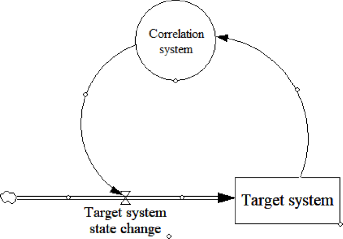
System dynamics integrates feedback theory and systems analysis with computer simulation to model complex systems, exploring how internal interactions between factors (positive/negative feedback) shape system behavior39. Changes in interconnected systems trigger material/energy exchanges, altering state variables that recursively influence system dynamics. This input–output interplay forms intricate feedback loops, jointly determining the system’s evolving state and behavioral patterns40,41,42. The schematic diagram is shown in Fig. 4 below.
The behavior of the system is determined by its structure, and the feedback loop is the basis of the structure. The study of causality is the basis of system dynamics. The causal relationship between variables within the system is represented by a straight line or arc with an arrow, called a causal chain. The positive causal chain is represented by + , and A change in the dependent variable (A) causes a change in the effect variable (B) in the same direction, Negative causal bonds are represented by −, where A change in the dependent variable (A) causes an inverse change in the effect variable (B)43,44. The schematic diagram is shown in Fig. 5 below.
Multiple causal chains are connected end to end to form a causal loop. The positive or negative of a causal loop depends on the number of negative causal chains in the loop45.


