
Algorithm verification
For evaluating the optimization performed by the NRBO algorithm, the authors chose four classical complex nonlinear benchmark functions as test cases for the iterative analysis. The results were compared and analyzed alongside two other algorithms: Differentiated Creative Search (DCS) and PID-based Search Optimization Algorithm (PSA). In this study, the population size of the algorithms was established at 20, while the maximum number of iterations was set to 500. For NRBO, the TOA determinant was established at DF = 0.6. In contrast, for PSA, the proportional coefficient was set to 1, while the integral coefficient was assigned a value of 0.5 and the differential coefficient was determined to be 1.2. The results of the function test are shown in Fig. 7.

It can be seen from Fig. 7 that the NRBO algorithm shows good convergence ability and speed in both single peak and multi peak benchmark test functions, and its convergence ability is significantly improved compared with DCS and PSA algorithms. It is evident that the algorithm demonstrates efficient exploratory capability, rapid convergence speed, and robust optimization performance.
NRBO-XGBoost combination model
XGBoost model has efficient training speed, strong extensibility and better prediction effect, but it takes up a large amount of computing resources and is vulnerable to the influence of super parameter selection. Low memory space and different combinations of super parameters may lead to different prediction results. To accurately and efficiently predict the stability of slopes in geotechnical engineering, the author employs the NRBO algorithm to optimize five critical parameters of the XGBoost model: maximum depth (max_depth), learning rate (learning_rate), subsample ratio (subsample), column sample ratio (colsample_bytree), and minimum loss (gamma). The specific implementation steps for the combined prediction model of geotechnical slope stability, optimized by XGBoost based on the NRBO algorithm, are outlined as follows.
-
a)
Data preprocessing. (1) The range of data distribution is reduced by standardizing the dimensions of unified data to eliminate the deviation of model prediction effect caused by data of different dimensions. (2) SMOTE algorithm is used to deal with the number of samples of slope instability, so that the two types of samples can reach a balance.
-
b)
NRBO initialization. Set the determination factor (TAO) to 0.6. The initial population size (pop_size) is 20. Set the maximum iteration threshold (max_iter) to 100. Set five super parameter optimization intervals.
-
c)
Find the best location. Optimization-seeking parameters are introduced into the objective function to update the fitness, the locations of the populations are refreshed according to the current state of the populations and the search rules, and the optimal solutions are updated using the root mean square error as a fitness function. After each iteration, the current optimal solution is used as a reference point for generating subsequent populations, and the fitness of each solution in the current population is evaluated until the stopping condition is recognized and the optimal parameter combination is output.
-
d)
Testing and application. The best combination of parameters after NRBO algorithm optimization is input into XGBoost model, and the best prediction model after training is obtained. The overall process of NRBO-XGBoost slope stability prediction model is shown in Fig. 8.
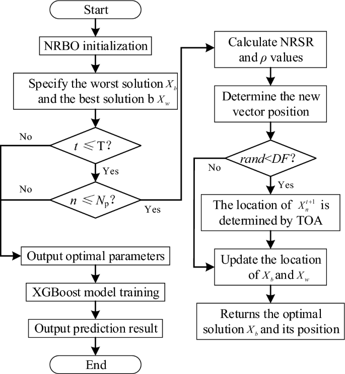
Flow of NRBO-XGBoost prediction model.
Model training and testing
Optimization of model parameters
After establishing the geotechnical engineering slope stability prediction model, 80% of the data from the original samples were randomly selected as the training set to train the model, while the remaining 20% were used as the test set to evaluate the model’s prediction performance. The training set consists of 198 samples, and the test set contains 50 samples, allowing for an assessment of the model’s feasibility, effectiveness, and robustness. Before super parameter optimization, it is necessary to comprehensively analyze the optimized super parameters and value range, as shown in Table 5.
The five hyperparameters of XGBoost model are optimized by NRBO algorithm to find the most suitable combination of hyperparameters with this model, and the dimension of NRBO algorithm is set to 5. Meanwhile, DCS and PSA are introduced to optimize the XGBoost model respectively, and compare the fitness situation of the above three algorithms individually. The results are illustrated in Fig. 9.

Fitness iteration curves for 3 optimization algorithms.
From Fig. 9, it is observed that the NRBO algorithm and DCS algorithm achieve a convergence value of 0.02 after 7 and 20 iterations for optimizing the hyperparameters of the XGBoost model, respectively, while the PSA algorithm requires 28 iterations to achieve a convergence value of 0.05. In contrast, the PSA algorithm requires 28 iterations to reach a higher convergence value of 0.05. This indicates that NRBO not only demonstrates superior optimization performance but also achieves lower convergence values compared to other intelligent algorithms. After optimization, the super parameter combination of the XGBoost model optimized by NRBO is learning_rate = 0.8247, max_depth = 7, sample = 0.6326, colsample_bytree = 0.6263 and gamma = 0.0758.
Model performance evaluation indicators
To validate the performance of the XGBoost slope stability prediction model after optimizing the NRBO algorithm, five metrics, namely Accuracy (Acc), Precision (Pre), Recall (Rec), F1 Score (Fs), and Coenkapa’s Coefficient (Ka), were introduced as a basis for evaluating the model performance35. The calculation process is as follows.
$$Acc = \frac{TP + TN}{{TP + TN + FP + FN}}$$
(10)
$$Pre = \frac{TP}{{TP + FP}}$$
(11)
$$Rec = \frac{TP}{{TP + FN}}$$
(12)
$$Fs = 2 \times \frac{Pre \times Rec}{{Pre + Rec}}$$
(13)
$$Ka = \frac{{N \cdot \sum\limits_{i = 1}^{n} {TP_{i} } – \sum\limits_{i = 1}^{n} {(TP_{i} + FP_{i} )(TP_{i} + FN_{i} )} }}{{N^{2} – \sum\limits_{i = 1}^{n} {(TP_{i} + FP_{i} )(TP_{i} + FN_{i} )} }}$$
(14)
where TP is the true case. TN is the true negative case. FP is the false positive case. FN is the false negative case. N is the total number of samples. n is the total number of sample categories.
Prediction effect analysis
To investigate further the robustness, superiority and robustness of the XGBoost slope stability prediction model optimized by the NRBO algorithm, the accuracy of the constructed model was evaluated in this study using the tenfold cross-validation method. The unoptimized XGBoost model as well as three models using DCS algorithm and PSA algorithm to optimize XGBoost respectively are selected and compared with the model built in the paper to analyze the difference in performance. The prediction performance of each model on the test set is shown in Table 6.
From Table 6, it can be seen that NRBO-XGBoost model predicts the slope stability compared with the actual stability, which is completely consistent with the actual state in the stable state of the slope, while there is a certain deviation in the destabilized state of the slope. It demonstrates that the model built in the paper has strong classification performance for the stable state of the slope and weak classification performance for the unstable state of the slope. Compared with the other 3 models, the NRBO-XGBoost model predicts the most correct slope stability state, which is 46, while DCS-XGBoost and PSA-XGBoost models were followed by 45 and 43 respectively, and the unoptimized XGBoost model predicted the least, 39. In order to intuitively understand the advantages of NRBO-XGBoost model, the comparison thermodynamic diagram of each evaluation index is drawn, as shown in Fig. 10.

Comparison of evaluation indicators of each prediction model.
It can be observed from Fig. 10 that the accuracy of NRBO-XGBoost slope stability accuracy model was increased by 2%, 6% and 14%, the precision was increased by 3.2%, 7.21% and 15.06%, the recall rate was increased by 1.9%, 5.93% and 14%, the F1-score was increased by 1.98%, 6% and 13.96%, and the Cohen’s Kappa coefficient was increased by 4.06%, 12.09% and 19%, respectively, compared with the evaluation indexes of DCS-XGBoost, PSA-XGBoost and XGBoost models. It is evident that the evaluation metrics of the NRBO-XGBoost slope stability prediction model surpass those of alternative models, indicating that this model demonstrates superior accuracy in predicting slope stability. To further verify the performance differences of the prediction models, the ROC curves and AUC values of NRBO-XGBoost, DCS-XGBoost, PSA-XGBoost and XGBoost slope stability prediction models are drawn, as shown in Fig. 11.

It is evident from Fig. 11 that the ROC curve of the NRBO-XGBoost slope stability prediction model is significantly extended towards the upper left corner, with an AUC value of 0.92 for the area under the curve. The ROC curves for the DCS-XGBoost and PSA-XGBoost prediction models show a secondary level of expansion, with AUC values of 0.90 and 0.85, respectively. In contrast, the non-optimized XGBoost prediction model exhibited the least favorable performance, achieving an AUC value of only 0.78. This analysis indicates that the NRBO-XGBoost model demonstrates superior predictive capability compared to other intelligent algorithm-based prediction models, which exhibit comparatively weaker performance.
Analysis of influencing factors
The causes of slope stability prediction are complex, and it is very important to identify the dominant disaster causing factors for the effective prevention and control strategy of slope instability. For this reason, the author uses the SHAP model to explain the importance of the six impact factors of the XGBoost model. The ranking of feature importance and the summary figure are shown in Fig. 12.

Feature importance ranking and overview.
Figure 12a shows the sequence of characteristic importance of slope stability state prediction, in which g, c, φ, H and j are the main factors affecting slope stability state, while ru has little effect. Each point in Fig. 12b represents a real sample, and the color of the point can reflect the size of the influencing factor value. According to the Shapley value of the given sample and the corresponding eigenvalue, the influence of the feature on the prediction result can be estimated. From a horizontal perspective, taking the influencing factors of g and c as examples, the sample distribution appears relatively scattered. This indicates that the influence of g and c on the model’s prediction results is substantial. In contrast, the influence factors φ, H, j, and ru are more concentrated, suggesting that their impact on the model’s prediction outcomes is comparatively minor. From a vertical standpoint, higher values of φ, h, and ru correspond to greater Shapley values. This implies that these factors have a more significant positive effect on predicting slope stability. Conversely, larger values of g, c, and j are associated with lower Shapley values; this indicates that these factors exert a stronger negative influence on predictions regarding slope stability. To sum up, the selected prediction indicators in this paper have an impact on slope instability, focusing on the influencing factors of g, c, φ, H and j, which can effectively prevent slope instability disasters to a large extent.

